3  Running McStas

This chapter describes usage of the McStas simulation package. In case of problems regarding installation or usage, the McStas mailing list [Mcs] or the authors should be contacted.

Performing a simulation using McStas can be divided into the following steps/elements

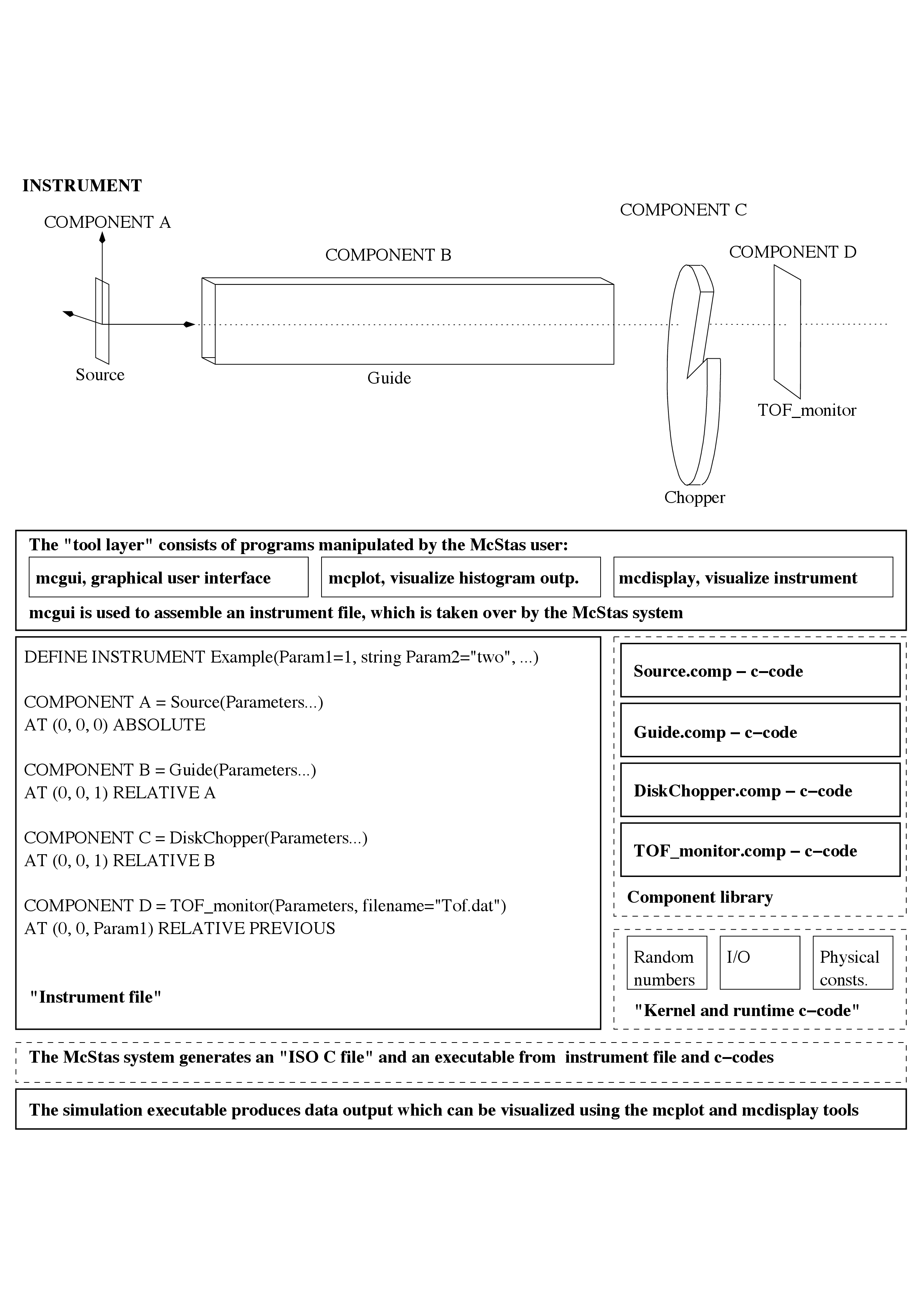
• The structure of McStas is illustrated in Figure 3.1.

• To use McStas, an instrument definition file describing the instrument to be simulated must be written. Alternatively, an example instrument file can be obtained from the examples/ directory in the distribution or from another source.

• The input files (instrument and component files) are written in the McStas meta-language and are edited either by using your favorite editor or by using the built-in editor of the graphical user interface (mcgui).

• Next, the McStas compiler mcstas is invoked to translate the instrument and component files into a C program. The program mcstas itself is written in C, using the parser flex and the compiler compiler bison.

• The resulting C program can then be compiled with a C compiler and run in combination with various front-end programs for example to present the intensity at the detector as a motor position is varied.

• The output data may be analyzed and visualized in the same way as regular experiments by using the data handling and visualization tools in McStas. As of McStas 3.x, these front-ends (mcplot, mcdisplay, mcresplot, …) are all implemented in Python, using matplotlib, pyqtgraph and browser/HTML (D3.js) back-ends, see section 3.5. Further data output formats including NeXus are available, see section 3.6.