Using MPI for parallel computing

3.7 Using MPI for parallel computing

Parallelizing a computation is in general possible when dependencies between each computation are not too strong. The situation of McStas is ideal since each neutron ray can be simulated without interfering with other simulated neutron rays. Therefore each neutron ray can be simulated independently on a set of computers.

When computing \(N\) neutron rays with \(p\) computers, each computer will simulate \(\frac {N}{p}\) neutrons. As a result there will be \(p \cdot \frac {N}{p} = N\) neutrons simulated. As a result, McStas generates two kinds of data sets:

intensity measurements, internally represented by three values \((p_0, p_1, p_2)\) where \(p_0\), \(p_1\), \(p_2\) are additive. Therefore the ﬁnal value of \(p_0\) is the sum of all local value of \(p_0\) computed on each node. The same rule applies for \(p_1\) and \(p_2\). The evaluation of the intensity errors \(\sigma \) is performed using the ﬁnal \(p_0\), \(p_1\), and \(p_2\) arrays (see Section 2.2.1).
event lists: the merge of events is done by concatenation

McStas provides two methods in order to distribute computations on many computers.

when using an homogeneous computer cluster, each simulation (including scan steps) may be computed in parallel using MPI. We recommend this method on clusters (see section 3.7.1).
mcrun’s built-in scan-splitting (--scan_split=N, see Table 3.1) distributes the individual steps of a parameter scan across N local CPU cores/threads, without requiring MPI. This is a lightweight alternative on a single multi-core machine.

All of these methods can be used, when available, from mcgui.

3.7.1 Parallel computing (MPI)

The MPI support requires that an MPI implementation (MPICH or OpenMPI are both known to work) is installed on a set of nodes, together with a properly conﬁgured passwordless ssh between nodes if running across more than one machine.

There are 2 methods for using MPI

Basic usage requires to compile and run the simulation by hand (mpicc, mpirun).
A much simpler way is to use mcrun -c --mpi=NB_CPU ... which will recompile and run with MPI support.
The McGUI interface also supports MPI from within the Run Dialog.

The MPI support is especially suited on clusters.

Requirements and limitation (MPI)

To use MPI you will need

A working MPI installation (MPICH or OpenMPI) on all nodes, and a McStas installation accessible from all nodes (e.g. on a shared ﬁlesystem, or installed identically on each node).
If running across more than one machine, ssh access between nodes without a password (e.g. using ssh-keygen and ssh-copy-id), and a machine list ﬁle (see --machines in Table 3.1).
Signals are not supported while simulating with MPI (since asynchronous events cannot be easily transmitted to all nodes). This means it is not possible to cancel an on-going computation. However, simulation scans can be interrupted as soon as the on-going computation step ends.

MPI Basic usage

To enable parallel computation, compile mcstas-generated C code with mpicc with the ﬂag -DUSE_MPI and run it using the wrapper of your MPI implementation (mpirun for mpich or lammpi) :

1  # generate a C-source file [sim.c] 
2  mcstas sim.instr 
3 
4  # generate an executable with MPI support [sim.mpi] 
5  mpicc -DUSE_MPI -o sim.mpi sim.c 
6 
7  # execute with parallel processing over <N> computers 
8  # here you have to list the computers you want to use 
9  # in a file [machines.list] (using mpich implementation) 
10  # (refer to MPI documentation for a complete description) 
11  mpirun -machinefile machines.list -n <N> \ 
12        ./sim.mpi <instrument parameters> 
13  ...
 
14

If you don’t want to spread the simulation, run it as usual:

1  ./sim.mpi <instrument parameters>
 
2

3.7.2 McRun options for MPI

The two relevant mcrun options are (see Table 3.1):

--mpi=<number>: tells mcrun to use MPI, and to spread the simulation over <number> nodes
--machines=<file>: deﬁnes a text ﬁle where the nodes which are to be used for parallel computation are listed, one node per line.

When available, the MPI option will show up in the mcgui Run dialog. Specify the number of nodes required.

Suppose you have four machines named node1 to node4. A typical machine list ﬁle, machines.list looks like :

1node1 
2node2 
3node3 
4node4

You can then spread a simulation sim.instr using mcrun :

1  mcrun -c --mpi=4 --machines=machines.list \ 
2        sim.instr <instrument parameters>
 
3

Warning: when using mcrun with MPI, be sure to recompile your simulation with MPI support (see -c ﬂag of mcrun): a simulation compiled without MPI support cannot be used with MPI, whereas a simulation compiled with MPI support can be used without MPI.

3.7.3 McStas/MPI Performance

Theoretically, a computation which lasts \(T\) seconds on a single computer, should lasts at least \(\frac {T}{p}\) seconds when it is distributed over \(p\) computers. In practice, there will be overhead time due to the split and merge operations.

the split is immediate: constant time cost \({\cal O}(1)\)
the merge is at worst linear against the number of computers:
- linear time cost : \({\cal O}(p)\) when saving an event list
- logarithmic time cost: \({\cal O}(\log {p})\) when not saving an event list

The eﬃciency of McStas using MPI has been tested on large clusters, up to 500 nodes. The computation time decreases in the same proportion as the number of nodes, showing an ideal eﬃciency. However, a small overhead may appear depending on the cluster internal network load, which may be estimated at most of about 10-20 s. This overhead comes from the spread and the fusion of the computations. For instance, spreading a computation implies often an rsh or and ssh session to be opened on every node. To reach the best eﬃciency, the computation time should not be lower than 30 seconds, or the overhead time may become signiﬁcant compared to total time.

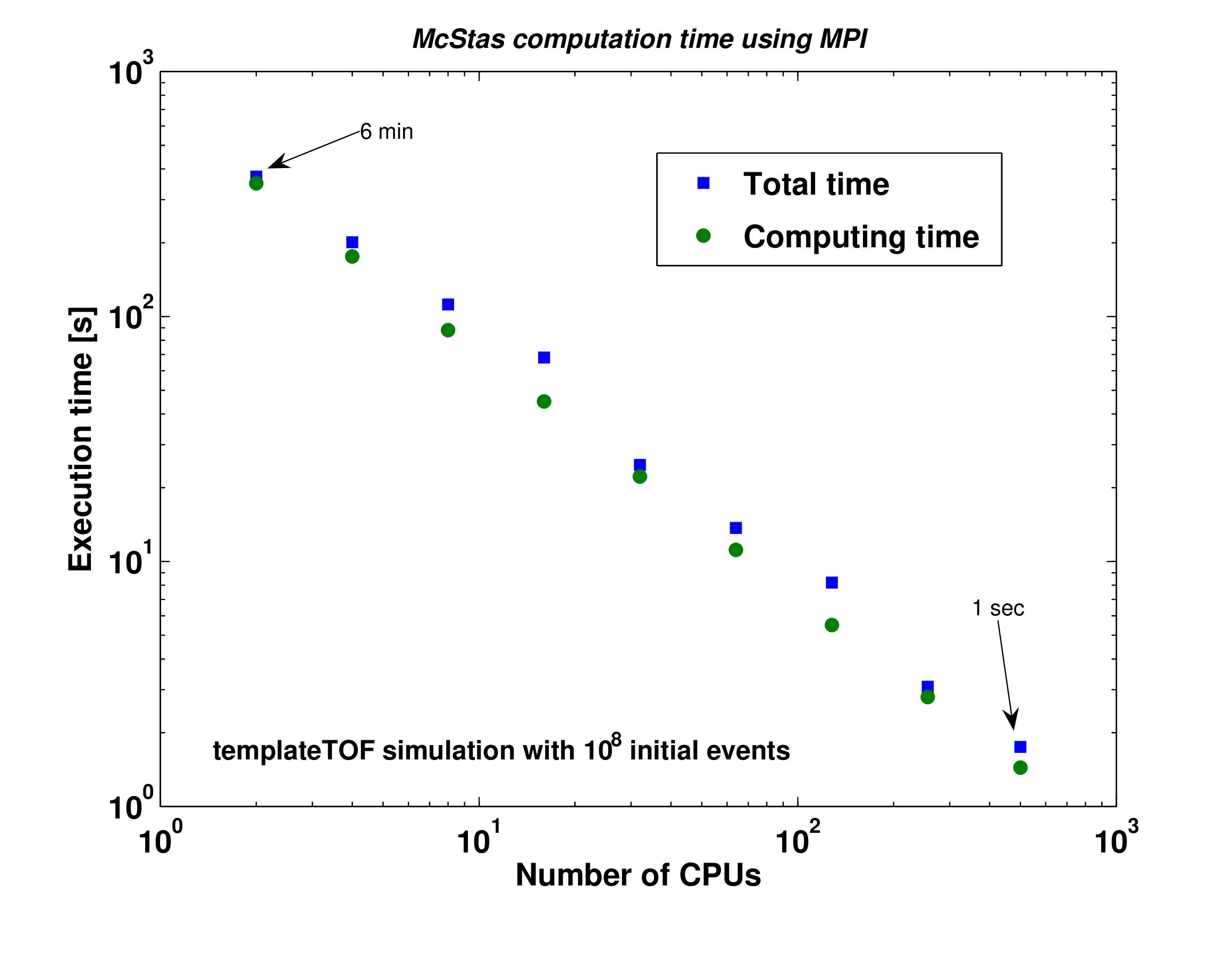
Figure 3.6.:

McStas/MPI execution time as a function of computing nodes, with templateTOF instrument and 1e8 initial neutron events. Tests performed on Lonestar@TACC (US Teragrid, 2008).

3.7.4 MPI Bugs and limitations

Some header of output ﬁles might contain minor errors.
The computation split does not take into account the speed or the load of nodes: the overall time of a distributed computation is forced by the slowest node; for optimal performance, the “cluster” should be homogeneous.
Interacting with a running simulation (USR1 and USR2 signals) is disabled with MPI.

[prev] [prev-tail] [front] [up]