8.3 The triple axis spectrometer TAS1
With this instrument definition, we have tried to create a very detailed model of the conventional cold-source triple-axis spectrometer TAS1 at the now closed neutron source DR3 of Risø National Laboratory. Except for the cold source itself, all components used have quite realistic properties. Furthermore, the overall geometry of the instrument has been adapted from the detailed technical drawings of the real spectrometer. The TAS 1 simulation was the first detailed work performed with the McStas package. For further details see reference [ACL98]. The instrument family lives under Risoe/ in the example library, e.g. Risoe/TAS1_Vana and Risoe/TAS1_Powder, and is also known by its historical name linup-* in older documentation.
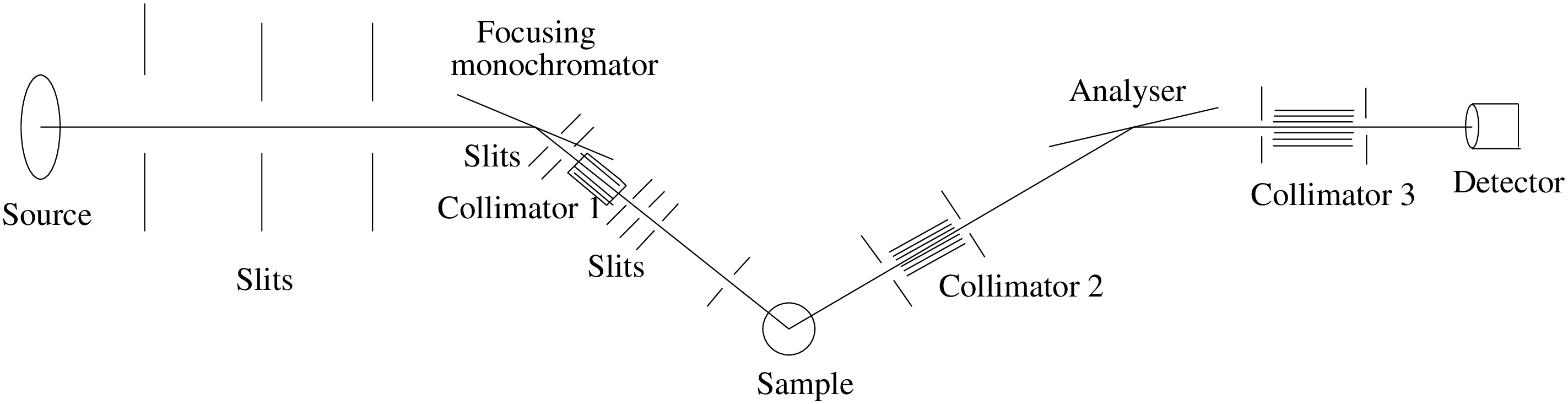
At the spectrometer, the channel from the cold source to the monochromator is asymmetric, since the first part of the channel is shared with other instruments. In the instrument definition, this is represented by three slits. For the cold source, we use a flat energy distribution (component Source_flat) focusing on the third slit.
The real monochromator consist of seven blades, vertically focusing on the sample. The angle of curvature is constant so that the focusing is perfect at 5.0 meV (20.0 meV for 2nd order reflections) for a 1\(\times \)1 cm\(^2\) sample. This is modeled directly in the instrument definition using seven Monochromator components. The mosaicity of the pyrolytic graphite crystals is nominally 30’ (FWHM) in both directions. However, the simulations indicated that the horisontal mosaicities of both monochromator and analyser were more likely 45’. This was used for all mosaicities in the final instrument definition.
The monochromator scattering angle, in effect determining the incoming neutron energy, is for the real spectrometer fixed by four holes in the shielding, corresponding to the energies 3.6, 5.0, 7.2, and 13.7 meV for first order neutrons. In the instrument definition, we have adapted the angle corresponding to 5.0 meV in order to test the simulations against measurements performed on the spectrometer.
The width of the exit channel from the monochromator may be narrowed down from initially 40 mm to 20 mm by an insert piece. In the simulations, we have chosen the 20 mm option and modeled the channel with two slits to match the experimental set-up.
In the test experiments, we used two standard samples: An Al\(_2\)O\(_3\) powder sample and a vanadium sample. The instrument definitions use either of these samples of the correct size. Both samples are chosen to focus on the opening aperture of collimator 2 (the one between the sample and the analyser). Two slits, one before and one after the sample, are in the instrument definition set to the opening values which were used in the experiments.
The analyser of the spectrometer is flat and made from pyrolytic graphite. It is placed between an entry and an exit channel, the latter leading to a single detector. All this has been copied into the instrument definition.
On the spectrometer, Soller collimators may be inserted at three positions: Between monochromator and sample, between sample and analyser, and between analyser and detector. In our instrument definition, we have used 30’, 28’, and 67’ collimators on these three positions, respectively.
An illustration of the TAS1 instrument is shown in figure 8.3. Test results and data from the real spectrometer are shown in Appendix 8.3.1.
8.3.1 Simulated and measured resolution of TAS1
In order to test the McStas package on a qualitative level, we have performed a very detailed comparison of a simulation with a standard experiment from TAS1. The measurement series constitutes a complete alignment of the spectrometer, using the direct beam and scattering from V and Al\(_2\)O\(_3\) samples at an incoming energy of 20.0 meV, using the second order scattering from the monochromator.
In these simulations, we have tried to reproduce every alignment scan with respect to position and width of the peaks, whereas we have not tried to compare absolute intensities. Below, we show a few comparisons of the simulations and the measurements.
Figure 8.4 shows a scan of \(2\theta _m\) on the collimated direct beam in two-axis mode. A 1 mm slit is placed on the sample position. Both the measured width and non-Gaussian peak shape are well reproduced by the McStas simulations.
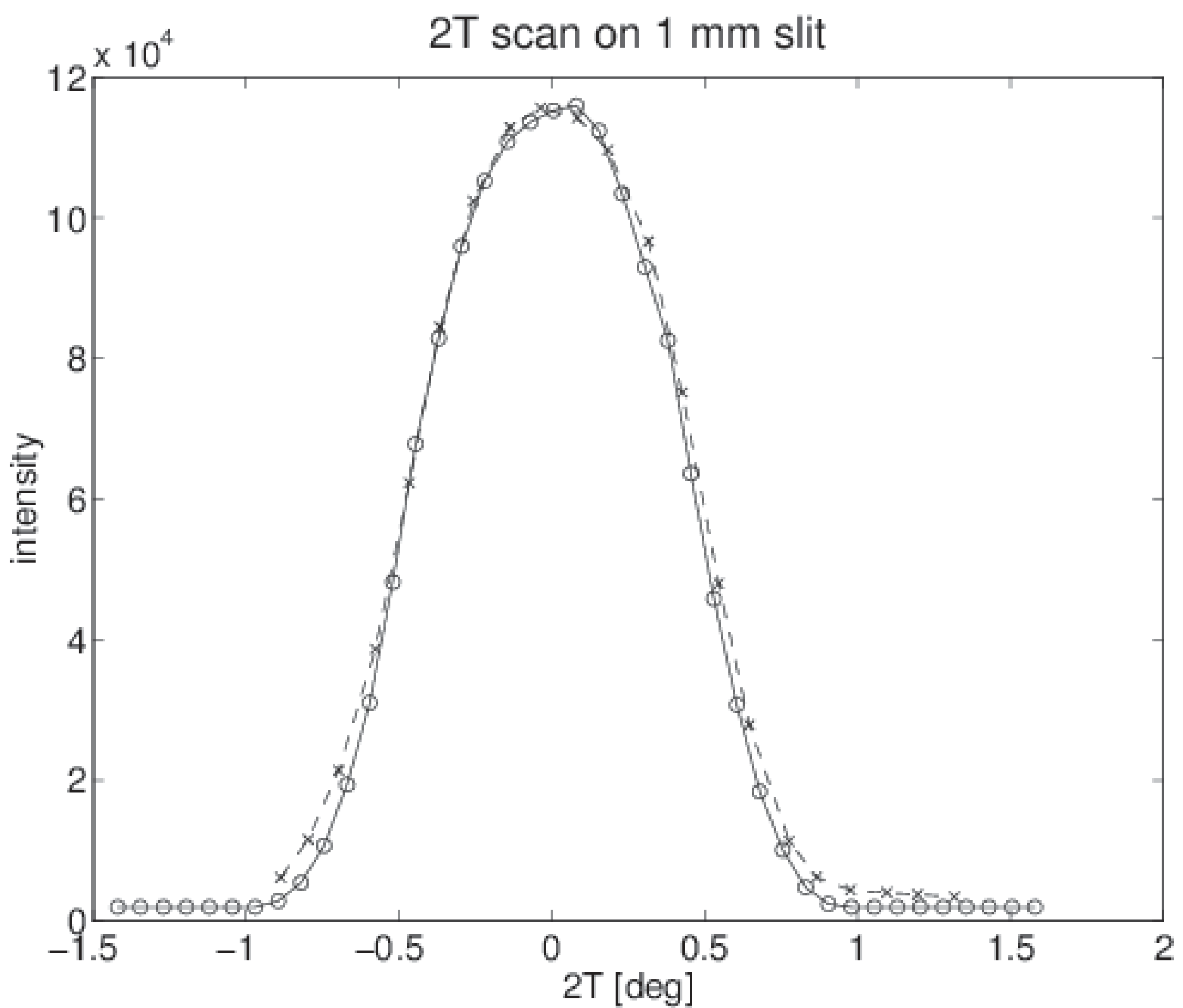
| Figure 8.4.: | TAS1: Scans of \(2\theta _s\) in the direct beam with 1 mm slit on the sample position. "\(\times \)": measurements, "o": simulations, scaled to the same intensity Collimations: open-30’-open-open. |
In contrast, a simulated \(2\theta _a\) scan in triple-axis mode on a V-sample showed a surprising offset from 0 degrees. However, a simulation with a PSD on the sample position showed that the beam center was 1.5 mm off from the center of the sample, and this was important since the beam was no wider than the sample itself. A subsequent centering of the beam resulted in a nice agreement between simulation and measurements. For a comparison on a slightly different instrument (analyser-detector collimator inserted), see Figure 8.5.
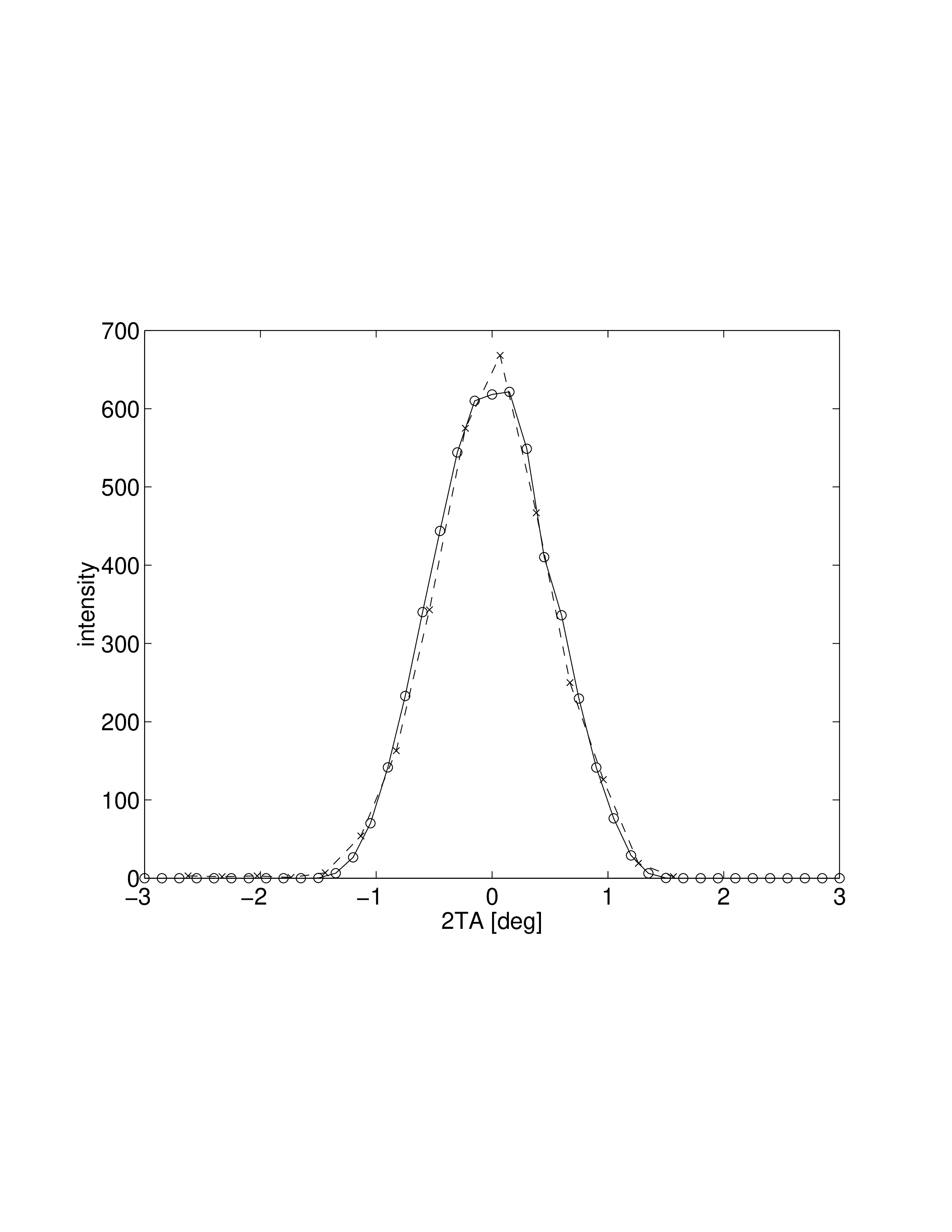
| Figure 8.5.: | TAS1: Corrected \(2\theta _a\) scan on a V-sample. Collimations: open-30’-28’-67’. "\(\times \)": measurements, "o": simulations. |
The result of a \(2\theta _s\) scan on an Al\(_2\)O\(_3\) powder sample in two-axis mode is shown in Figure 8.6. Both for the scan in focusing mode (+ \(-\) +) and for the one in defocusing mode (+ + +) (not shown), the agreement between simulation and experiment is excellent.
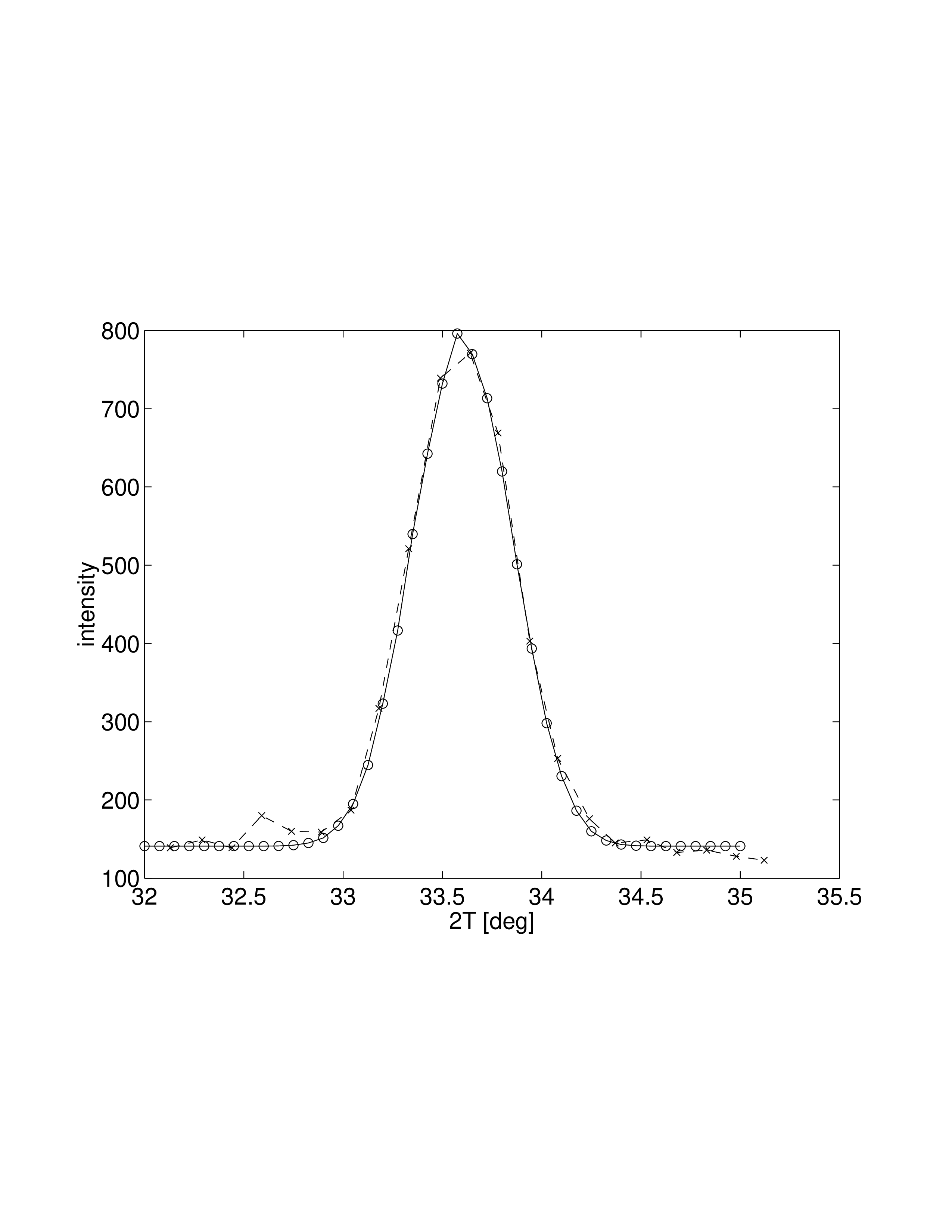
| Figure 8.6.: | TAS1: \(2\theta _s\) scans on Al\(_2\)O\(_3\) in two-axis, focusing mode. Collimations: open-30’-28’-67’. "\(\times \)": measurements, "o": simulations. A constant background is added to the simulated data. |
As a final result, we present a scan of the energy transfer \(E_a = \hbar \omega \) on a V-sample. The data are shown in Figure 8.7.
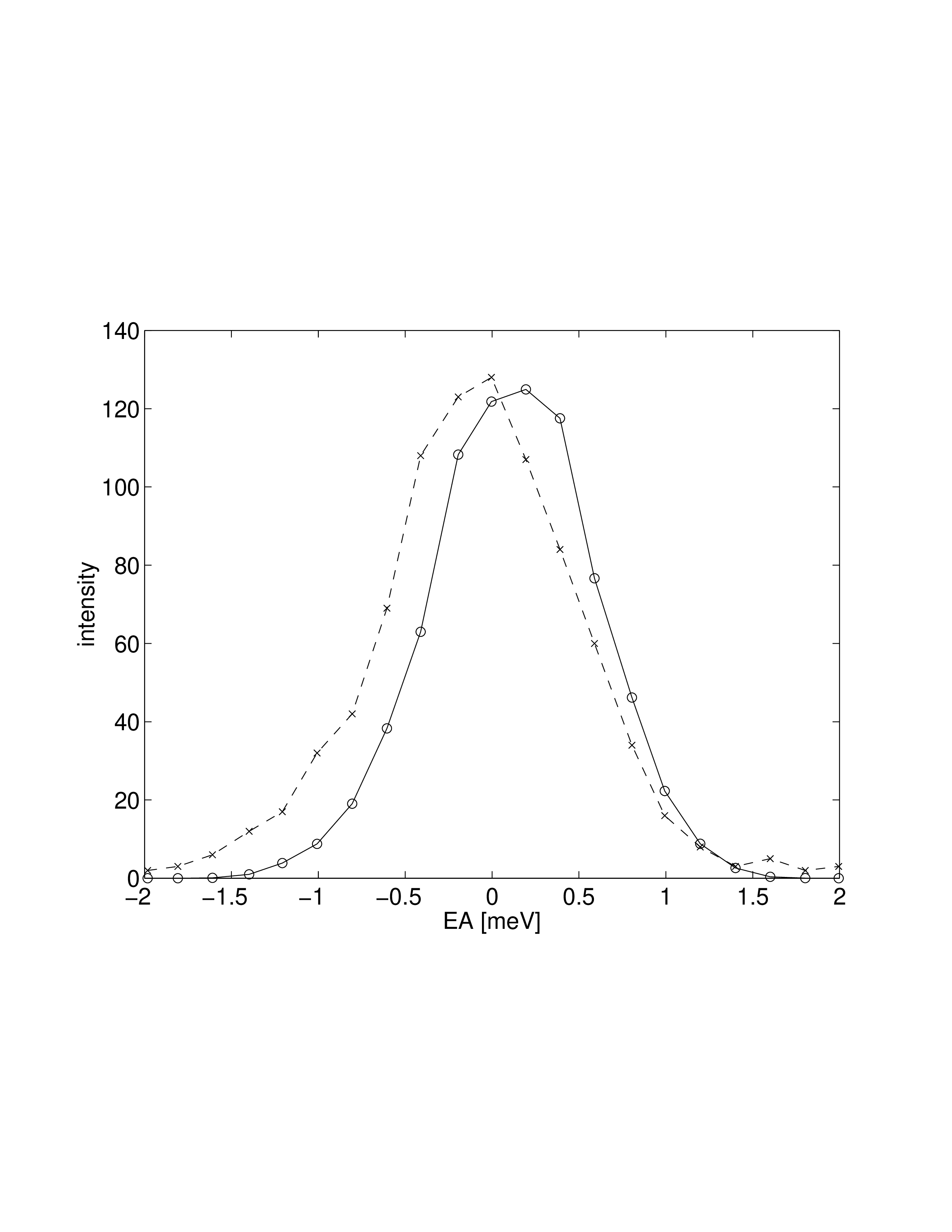
| Figure 8.7.: | TAS1: Scans of the analyser energy on a V-sample. Collimations: open-30’-28’-67’. "\(\times \)": measurements, "o": simulations. |
For a modern triple-axis instrument that is not tied to a specific, decommissioned facility, see the Templates/templateTAS example instead, which additionally includes a basic in-plane UB-matrix transformation useful for estimating resolution functions of an arbitrary TAS configuration (see also mcresplot, section 3.5.6).