3.2  Brief introduction to the graphical user interface

This section gives an ultra-brief overview of how to use McStas once it has been properly installed. It is intended for those who do not read manuals if they can avoid it. For details on the different steps, see the following sections. This section uses the BNL_H8.instr file supplied in the examples/BNL/BNL_H8 directory of the McStas distribution.

To start the graphical user interface of McStas, run the mcgui command which will open a window with a number of menus, see figure 3.2.

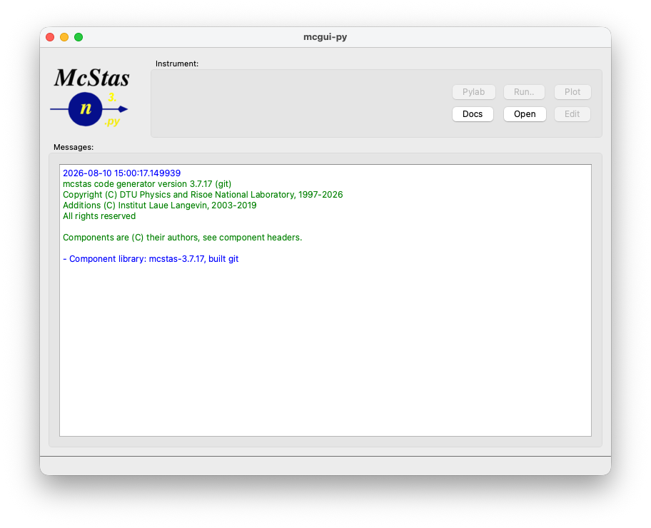
To load an instrument, select “New from Template” (formerly known as the “Neutron site” menu) and open the template/example BNL/BNL_H8. Next, check that the current plotting backend setting (“Preferences” in the File menu, or the --autoplotter option of mcrun) corresponds to your system setup:

• by editing the user configuration file, see mcrun --edit-user-config,

Next, select “Run simulation” from the “Simulation” menu. The McStas compiler mcstas will translate the definition into an executable program. Then mcgui will pop up a dialog window. Type a value for the “ROT” parameter (e.g. 90), check the “Plot results” option, and select “Start”. The simulation will run, and when it finishes after a while the results will be plotted in a window, using one of the Python plotting back-ends (matplotlib, pyqtgraph or an HTML/browser view), see section 3.5.5. For other options, execute mcplot --help to get help.

To visualize or debug the simulation graphically, repeat the steps but check the “Trace” option instead of the “Simulate” option. A window will pop up showing a sketch of the instrument, drawn by the mcdisplay front-end (section 3.5.4), again using one of the matplotlib, pyqtgraph or webGL back-ends.

For a slightly longer gentle introduction to McStas, see the McStas tutorial (available from [Mcs]), and as of version 3.8.6 built into the mcgui help menu. For more technical details, read on from section 3.3