Polarized Neutron Scattering

5.2 Polarized Neutron Scattering

First we will give a short introduction to how calculations are done and then quote some results which are important for implementing the ﬁrst McStas components.

All the potentials (nuclear, magnetic, and electric) we will be interested in can be written on the form: \begin {equation} \label {eq:general_pot} \hat {v} = \betao + \alphao \cdot \sigmao \end {equation}

The ﬁrst term does not aﬀect the spin, while the second term can change the spin. Let us just remind here that:

\begin {equation} \label {eq:pauli_rules} \begin {matrix} \sigmaH _x \chiU = \chiD , & \sigmaH _y \chiU = i\chiD , & \sigmaH _z \chiU = \chiU , \\ \sigmaH _x \chiD = \chiU , & \sigmaH _y \chiD = -i\chiU , & \sigmaH _z \chiD = -\chiD . \end {matrix} \end {equation}

So that the interaction proportional to \(\sigmaH _x\) and \(\sigmaH _y\) results in spin ﬂips, while the interactions with \(\sigmaH _z\) conserves the spin.

It turns out to be smart to deﬁne a density matrix operator: \begin {equation} \rhoo = \chi \chi ^\dagger = \left ( \begin {matrix} |a|^2 & ab^\ast \\ ba^\ast & |b|^2 \end {matrix} \right ) = \frac {1}{2}({\cal I}+\PB \cdot \sigmao ), \end {equation} where \(\chi \) is the neutron wave function (Eq. 5.5), and \(\cal I\) is the unit matrix.

Using the density matrix the elastic cross section can be written as ([Lov84], Eq. 10.31): \begin {equation} \label {eq:master_sigma} \frac {d\sigma }{d\Omega } = \text {Tr} \rhoo \hat {v}^\dagger \hat {v} = \sum _{\lambda , \lambda '} p_\lambda \text {Tr} \rhoo \langle \lambda | \hat {V}^\dagger (\Q ) | \lambda ' \rangle \langle \lambda ' | \hat {V}(\Q ) | \lambda \rangle \delta (E_\lambda - E_{\lambda '}), \end {equation}

where \(\hat {V}\) is the interaction potential and it is understood that the trace is to be taken with respect only to the neutron spin coordinates. The outgoing polarization is given as: \begin {equation} \label {eq:master_pol} \PB ' \frac {d\sigma }{d\Omega } = \text {Tr} \rhoo \hat {v}^\dagger \sigmao \hat {v} = \sum _{\lambda , \lambda '} p_\lambda \text {Tr} \rhoo \langle \lambda | \hat {V}^\dagger (\Q ) | \lambda ' \rangle \sigmao \langle \lambda ' | \hat {V}(\Q ) | \lambda \rangle \delta (E_\lambda - E_{\lambda '}) \end {equation}

Inserting Eq. 5.12 in Eq. 5.15 and Eq. 5.16 results in the two master equations for polarized neutron scattering:

\begin {equation} \label {eq:general_sigma} \text {Tr} \rhoo \hat {v}^\dagger \hat {v} = \alphao ^\dagger \cdot \alphao + \betao ^\dagger \betao + \betao ^\dagger (\alphao \cdot \PB ) + (\alphao ^\dagger \cdot \PB ) \betao + i\PB \cdot (\alphao ^\dagger \times \alphao ), \end {equation}

and

\begin {equation} \label {eq:general_pol} \text {Tr} \rhoo \hat {v}^\dagger \sigmao \hat {v} = \betao ^\dagger \alphao + \alphao ^\dagger \betao + \betao ^\dagger \betao \PB + \alphao ^\dagger (\alphao \cdot \PB ) + (\alphao ^\dagger \cdot \PB ) \alphao - \PB (\alphao ^\dagger \cdot \alphao ) - i \alphao ^\dagger \times \alphao + i \betao ^\dagger (\alphao \times \PB ) + i (\PB \times \alphao ^\dagger ) \betao . \end {equation}

Based on these two equations and the interaction potentials all the results presented in the following are derived in [Lov84].

5.2.1 Example: Nuclear scattering

The nuclear scattering potential for a crystal is: \begin {equation} \label {eq:nuclear_pot} \hat {V}_N(\Q ) = \sum _{\lB ,\dB } \exp (i\Q \cdot \RB _{ld})(A_{ld} + \frac {1}{2} B_{ld} \sigmao \cdot \Io _{ld}), \end {equation}

so that

\begin {eqnarray} \label {eq:ab_nuclear} \alphao & = & \sum _{\lB ,\dB } \exp (i\Q \cdot \RB _{ld}) \frac {1}{2} B_{ld} \Io _{ld} \\ \betao & = & \sum _{\lB ,\dB } \exp (i\Q \cdot \RB _{ld}) A_{ld}, \end {eqnarray}

where \(\Io \) is the nuclear spin operator and the constants \(A\) and \(B\) are related to the nuclear scattering lengths \(b^+\) and \(b^-\) as \(A=((I+1)b^++Ib^-)/(2I+1)\) and \(B=(b^++b^-)/(2I+1)\).

To calculate the polarization cross section and outgoing polarization we have to average over the nuclear spin (which we assume is random oriented), so that terms linear in \(\alphao \) (three last terms in Eq. 5.17) disappears. The scattering cross section ends up being (see [Lov84] p. 159):

\begin {equation} \label {eq:nuclear_sigma} \frac {d\sigma }{d\Omega } = \sum _{\lB , \dB , \lB ', \dB '} \exp (i \Q \cdot (\RB _{ld}-\RB _{l'd'})) (\madsq + \delta _{\lB ,\lB '}\delta _{\dB ,\dB '}[\sqmad - \madsq + \frac {1}{4}\bd ]) \end {equation}

where the ﬁrst term is the coherent cross-section and the second term is the site-incoherent cross-section. Both terms are independent of \(\PB \) as expected for a system without a preferred internal direction.

The polarization in the ﬁnal state is:

\begin {equation} \label {eq:nuclear_pol} \PB ' \frac {d\sigma }{d\Omega } = \sum _{\lB , \dB , \lB ', \dB '} \exp (i \Q \cdot (\RB _{ld}-\RB _{l'd'})) \PB ' (\madsq + \delta _{\lB ,\lB '}\delta _{\dB ,\dB '}[\sqmad - \madsq - \frac {1}{12}\bd ]) \end {equation}

Comparing Eq. 5.20 and Eq. 5.21 we ﬁnd that: 1) The nuclear coherent polarization is the same as the initial polarization. 2) The same is true for the incoherent scattering due to the random isotope distribution. 3) The nuclear incoherent scattering due to the random nuclear spin orientations has polarization \(\PB ' = -1/3 \PB \) (for a random nuclear spin the associated Pauli matrix will 2/3 of the time point in the direction of \(\sigmaH _x\) and \(\sigmaH _y\) which according to Eq. 5.13 ﬂips the spin).

For Vanadium, where there is only one isotope and coherent scattering is negligible, we ﬁnd \(\PB ' = -1/3\PB \). There is however one catch. If the probability for multiple scattering is large one has to take into account that after two scattering one has: \(\PB '(2) = 1/9\PB \), and so forth. The average polarization after a thick vanadium target is therefore a sum of diﬀerent contributions.

5.2.2 Example: Polarizing Monochromator and Guides

Figure 5.1.:

Principle and geometry of a polarizing monochromator.

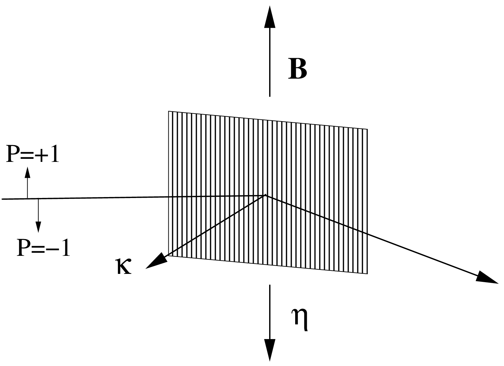
In a polarized monochromator and polarizing guides we have a ferromagnetic crystal in an external magnetic ﬁeld. The scattering potential is now both nuclear (no internal direction) and magnetic (internal direction), so in general the outgoing polarization can be quite complex. However, as illustrated in Figure 5.1, the typical setup has many geometrical constraints: \(\tN \cdot \tQ = 0\), \(\tN \cdot \PB _\perp = \tN \cdot \PB \), and \(\Q \times (\tN \times \Q ) = \tN \), which simpliﬁes the problem.

In [Lov84] the calculation for a centrosymmetric ferromagnetic crystal is done, and inserting the constraints above one ﬁnds ([Lov84], Eq. 10.96 and Eq. 10.110):

\begin {eqnarray} \label {eq:mono_sigma} d\sigma /d\Omega & = & \FN ^2 + 2\FN \FM (\PB \cdot \tN ) + \FM ^2\\ \label {eq:mono_pol} \PB ' d\sigma /d\Omega & = & \PB [\FN ^2 - \FM ^2] + \tN [2\FN \FM + 2(\tN \cdot \PB )\FM ^2] \end {eqnarray}

NB! Note that in [Wil88] Eq. 2.2.25 there is a minus in front of the second term in Eq. ??. We have not been able to understand this discrepancy, which is probably due to notation. Most other authors agree with the minus in front of the second term (e.g. Squires and Francis Tasset).

For a beam which is initially unpolarized we ﬁnd the outgoing polarization to be: \begin {equation} \PB ' = \frac {\tN 2\FN \FM }{d\sigma /d\Omega } = \frac {2\FN \FM }{\FN ^2 + \FM ^2} \tN , \end {equation}

so that the beam is fully polarized along \(\tN \) if \(\FN = \pm \FM \).

What we use to characterize the polarizing monochromator in practice is not \(\FN \) and \(\FM \), but instead the reﬂection probabilities \(\Ru \) and \(\Rd \) (for the reﬂection of interest).

If we assume that the reﬂection probabilities are directly proportional to the cross sections (with proportionality constant \(k\)), i.e., \(\Ru = k d\sigma /d\Omega (\PB =+\tN )\) and \(\Rd = k d\sigma /d\Omega (\PB =-\tN )\) then we can use Eq. ?? to determine \(\FN \) and \(\FM \):

\begin {eqnarray} \label {eq:mono_up} \Ru & = & k (\FN + \FM )^2,\\ \label {eq:mono_down} \Rd & = & k (\FN - \FM )^2. \end {eqnarray}

The values of \(\sqrt {k}\FN \) and \(\sqrt {k}\FM \) are then between -1 and +1 and unit less like the reﬂection probabilities. In the following we ignore \(k\) and just talk about \(\FN \) and \(\FM \).

In principle there are four solutions for \(\FN \) and \(\FM \), so in the code we currently choose the values where \(\FN + \FM = +\sqrt {\Ru }\) and \(\FN - \FM = +\sqrt {\Rd }\) (so that \(\FN >0\) and \(\FN >\FM \)). We then ﬁnd:

\begin {eqnarray} \label {eq:mono_nuc} \FN & = & \frac {\sqrt {\Ru } + \sqrt {\Rd }}{2},\\ \label {eq:mono_mag} \FM & = & \frac {\sqrt {\Ru } - \sqrt {\Rd }}{2}. \end {eqnarray}

When \(\FN \) and \(\FM \) are determined from these equations, Eq. ?? and Eq. ?? can easily be used to handle any situation.

This solution is both used for monochromators and guides.

It is not clear that this solution is correct. If we make a simple example with \(\Ru = 1\) and \(\Rd = 0.25\) then we could in principle have four solutions, but let us just quote the two where \(\FN \) is positive since the last two are found by inserting a minus before all the solutions and this does not change the physics. The two solutions are \(\FN = 0.75, \FM =0.25\) and \(\FM = 0.75, \FN =0.25\). All solutions gives the same cross section, but if the incoming beam is polarized (and only then) the outgoing beam will have two diﬀerent polarization values, since \(\PB [\FN ^2 - \FM ^2]\) and \(\tN 2(\tN \cdot \PB )\FM ^2\) are diﬀerent for the two solutions. It seems that one needs some additional information to choose between the two solutions.

NB! The simplifying geometry shown in Figure 5.1 only applies for the sides of the guide wall and not the top and bottom (assuming that the magnetizing ﬁeld is pointing up or down), so there another set of equations should really be used.

The same physics could also be used for a polarizing powder or single crystal sample if \(\FN \) and \(\FM \) can be calculated with some other program, but one would have to use the general form of Eq. ?? and Eq. ?? without the simplifying geometrical constraints for monochromators and guides.

[next] [prev] [prev-tail] [front] [up]