3 Source components
McStas contains a number of different source components, and any simulation will usually contain exactly one of these sources. The main function of a source is to determine a set of initial parameters \((\textbf {r}, \textbf {v}, t)\) for each neutron ray. This is done by Monte Carlo choices from suitable distributions. For example, in most present sources the initial position is found from a uniform distribution over the source surface, which can be chosen to be either circular or rectangular. The initial neutron velocity is selected within an interval of either the corresponding energy or the corresponding wavelength. Polarization is not relevant for sources, and we initialize the neutron average spin to zero: \(\textbf {s}=(0,0,0)\).
For time-of-flight sources, the choice of the emission time, \(t\), is being made on basis of detailed analytical expressions. For other sources, \(t\) is set to zero. In the case one would like to use a steady state source with time-of-flight settings, the emission time of each neutron ray should be determined using a Monte Carlo choice. This may be achieved by the EXTEND keyword in the instrument description source as in the example below:
1  TRACE
2
3  COMPONENT MySource=Source_gen(...) AT (...)
4  EXTEND
5  %{
6    t = 1e-3*randpm1(); /* set time to +/- 1 ms */
7  %}
3.1 The Source_simple McStas Component
Identification
Description
Input parameters
Links
A simple continuous source with a flat energy/wavelength spectrum
3.2 The Source_div McStas Component
Identification
Description
Input parameters
Links
A continuous source with specified divergence
3.3 The Source_Maxwell_3 McStas Component
Identification
Description
Input parameters
Links
A continuous source with a Maxwellian spectrum
3.4 The Source_gen McStas Component
Identification
Description
Input parameters
Links
A general continuous source
3.5 The Moderator McStas Component
Identification
Description
Input parameters
Links
A time-of-flight source (pulsed)
3.6 The Source_adapt McStas Component
Identification
Description
Input parameters
Links
A neutron source with adaptive importance sampling
3.7 The Adapt_check McStas Component
Identification
Description
Input parameters
Links
The adaptive importance sampling monitor
3.8 The Source_Optimizer McStas Component
Identification
Description
Input parameters
Links
A general Optimizer for McStas
3.9 The Monitor_Optimizer McStas Component
Identification
Description
Input parameters
Links
Optimization locations for the Source_Optimizer
3.10 Other sources components: contributed pulsed sources, virtual sources (event files)
3.0.1 Neutron flux
The flux of the sources deserves special attention. The total neutron intensity is defined as the sum of weights of all emitted neutron rays during one simulation (the unit of total neutron weight is thus neutrons per second). The flux, \(\psi \), at an instrument is defined as intensity per area perpendicular to the beam direction.
The source flux, \(\Phi \), is defined in different units: the number of neutrons emitted per second from a 1 cm\(^2\) area on the source surface, with direction within a 1 ster. solid angle, and with wavelength within a 1 Å interval. The total intensity of real neutrons emitted towards a given diaphragm (units: n/sec) is therefore (for constant \(\Phi \)): \begin {equation} I_\textrm {total} = \Phi A \Delta \Omega \Delta \lambda , \end {equation} where \(A\) is the source area, \(\Delta \Omega \) is the solid angle of the diaphragm as seen from the source surface, and \(\Delta \lambda \) is the width of the wavelength interval in which neutrons are emitted (assuming a uniform wavelength spectrum).
The simulations are performed so that detector intensities are independent of the number of neutron histories simulated (although more neutron histories will give better statistics). If \(N_\textrm {sim}\) denotes the number of neutron histories to simulate, the initial neutron weight \(p_0\) must be set to \begin {equation} \label {proprule} p_0 = \frac {N_\textrm {total}}{N_\textrm {sim}} = \frac {\Phi (\lambda )}{N_\textrm {sim}} A \Omega \Delta \lambda , \end {equation} where the source flux is now given a \(\lambda \)-dependence.
As a start, we recommend new McStas users to use the Source_simple component. Slightly more realistic sources are Source_Maxwell_3 for continuous sources or Moderator for time-of-flight sources.
Optimizers can dramatically improve the statistics, but may occasionally give wrong results, due to misleaded optimization. You should always check such simulations with (shorter) non-optimized ones.
Other ways to speed-up simulations are to read events from a file. See section 3.10 for details.
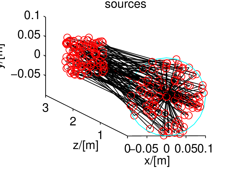
| Figure 3.1.: | A circular source component (at z=0) emitting neutron events randomly, either from a model, or from a data file. |