9.4 The Single_crystal McStas Component
Mosaic single crystal with multiple scattering vectors, optimised for speed with large crystals and many reflections.
Identification
-
Author: Kristian Nielsen
-
Origin: Risoe
-
Date: December 1999
Description
Single crystal with mosaic. Delta-D/D option for finite-size effects. Rectangular geometry. Multiple scattering and secondary extinction included. The mosaic may EITHER be specified isotropic by setting the mosaic input parameter, OR anisotropic by setting the mosaic_a, mosaic_b, and mosaic_c parameters. The crystal lattice can be bent locally, keeping the external geometry unchanged. Curvature is spherical along vertical and horizontal axes.
Speed/stat optimisation using SPLIT In order to dramatically improve the simulation efficiency, we recommend to use a SPLIT keyword on this component (or prior to it), as well as to disable the multiple scattering handling by setting order=1. This is especially powerful for large reflection lists such as with macromolecular proteins. When an incoming particle is identical to the preceeding, reciprocal space initialisation is skipped, and a Monte Carlo choice is done on available reflections from the last repciprocal space calculation! To assist the user in choosing a "relevant" value of the SPLIT, a rolling average of the number of available reflections is calculated and presented in the component output.
Mosacitiy modes: The component features three independent ways of parametrising mosaicity: a) The original algorithm where mosaicity is implemented by extending each reflection by a Gaussian "cigar" in reciprocal space, characterised by the parameters mosaic and delta_d_d. (Also known as "isotropic mosaicity".) b) A similar mode where mosaicities can be non-isotropic and given as the parameters mosaic_a, mosaic_b and mosaic_c, around the unit cell axes. (Also known as "anisotropic mosaicity".) c) Given two "macroscopically"/experimentally measured width/mosaicities of two independent reflections, parametrised by the list mosaic_AB = {mos_a, mos_b, a_h, a_k, a_l, b_h, b_k, b_l}, a set of microscopic mosaicities as in b) are estimated (internally) and applied. (Also known as "phenomenological mosaicity".)
Powder- and PG-mode When these two modes are used (powder=1 or PG=1), a randomised transformation of the particle direction is made before and after scattering, thereby letting the single crystal behave as a crystallite of either a powder (crystallite orientation fully randomised) or pyrolytic graphite (crystallite randomised around the c-axis).
Curved crystal mode The component features a method to curve the lattice planes slightly with respect to the outer geometry of the crystal. The method is implemented as a transformation on the particle direction vector, and should be used only in cases where a) The reflection lattice vector is ~ orthogonal to the crystal surface b) The modelled curvarture is "small" with respect to the crystal surface
Sample shape: Sample shape may be a cylinder, a sphere, a box or any other shape
box/plate:       xwidth x yheight x zdepth
cylinder:        radius x yheight
sphere:          radius (yheight=0)
any shape:       geometry=OFF file
The complex geometry option handles any closed non-convex polyhedra. It computes the intersection points of the neutron ray with the object transparently, so that it can be used like a regular sample object. It supports the PLY, OFF and NOFF file format but not COFF (colored faces). Such files may be generated from XYZ data using: qhull < coordinates.xyz Qx Qv Tv o > geomview.off or powercrust coordinates.xyz and viewed with geomview or java -jar jroff.jar (see below). The default size of the object depends on the OFF file data, but its bounding box may be resized using xwidth,yheight and zdepth.
Crystal definition file format Crystal structure is specified with an ascii data file. Each line contains 4 or more numbers, separated by white spaces:
h k l ... F2
The first three numbers are the (h,k,l) indices of the reciprocal lattice point, and the 7-th number is the value of the structure factor |F|**2, in barns. The rest of the numbers are not used; the file is in the format output by the Crystallographica program. The reflection list should be ordered by decreasing d-spacing values. Lines begining by ’#’ are read as comments (ignored). Most sample parameters may be defined from the data file header, following the same mechanism as PowderN.
Current data file header keywords include, for data format specification: #column_h <index of the Bragg Qh column> #column_k <index of the Bragg Qk column> #column_l <index of the Bragg Ql column> #column_F2 <index of the squared str. factor ’|F|^2’ column [b]> #column_F <index of the structure factor norm ’|F|’ column> and for material specification: #sigma_abs <value of absorption cross section [barns]> #sigma_inc <value of incoherent cross section [barns]> #Delta_d/d <value of Detla_d/d width for all lines> #lattice_a <value of the a lattice parameter [Å]> #lattice_b <value of the b lattice parameter [Å]> #lattice_c <value of the c lattice parameter [Å]> #lattice_aa <value of the alpha lattice angle [deg]> #lattice_bb <value of the beta lattice angle [deg]> #lattice_cc <value of the gamma lattice angle [deg]>
Last, CIF, FullProf and ShelX files can be read, and converted to F2(hkl) lists if ’cif2hkl’ is installed. The CIF2HKL env variable can be used to point to a proper executable, else the McCode, then the system installed versions are used.
See the Component Manual for more defails.
Example: Single_crystal(xwidth=0.01, yheight=0.01, zdepth=0.01, mosaic = 5, reflections="YBaCuO.lau")
A PG graphite crystal plate, cut for (002) reflections Single_crystal(xwidth = 0.002, yheight = 0.1, zdepth = 0.1, mosaic = 30, reflections = "C_graphite.lau",
ax=0,      ay=2.14,   az=-1.24,
bx = 0,    by = 0,    bz =  2.47,
cx = 6.71, cy = 0,    cz =  0)
A leucine protein, without multiple scattering Single_crystal(xwidth=0.005, yheight=0.005, zdepth=0.005, mosaic = 5, reflections="leucine.lau", order=1)
A Vanadium incoherent elastic scattering with multiple scattering Single_crystal(xwidth=0.01, yheight=0.01, zdepth=0.01, reflections="", sigma_abs=5.08, sigma_inc=4.935,
ax=3.0282, by=3.0282, cz=3.0282/2)
Also, always use a non-zero value of delta_d_d.
%VALIDATION: This component has been validated.
This sample component can advantageously benefit from the SPLIT feature, e.g. SPLIT COMPONENT sx = Single_crystal(...)
Input parameters
Parameters in boldface are required; the others are optional.
|
Name |
Unit |
Description |
Default |
|
|
|||
|
reflections |
string |
File name containing structure factors of reflections (LAZ LAU CIF, FullProf, ShelX). Use empty ("") or NULL for incoherent scattering only |
0 |
|
geometry |
str |
Name of an Object File Format (OFF) or PLY file for complex geometry. The OFF/PLY file may be generated from XYZ coordinates using qhull/powercrust |
0 |
|
mosaic_AB |
arc_minutes, arc_minutes,1, 1, 1, 1, 1, 1 |
In Plane mosaic rotation and plane vectors (anisotropic), mosaic_A, mosaic_B, A_h,A_k,A_l, B_h,B_k,B_l. Puts the crystal in the in-plane mosaic state. Vectors A and B define plane in which the crystal roation is defined, and mosaic_A, mosaic_B, denotes the resp. mosaicities (gaussian RMS) with respect to the two reflections chosen by A and B (Miller indices). |
{0,0, 0,0,0, 0,0,0} |
|
xwidth |
m |
Width of crystal |
0 |
|
yheight |
m |
Height of crystal |
0 |
|
zdepth |
m |
Depth of crystal (no extinction simulated) |
0 |
|
radius |
m |
Outer radius of sample in (x,z) plane |
0 |
|
delta_d_d |
1 |
Lattice spacing variance, gaussian RMS |
1e-4 |
|
mosaic |
arc minutes |
Crystal mosaic (isotropic), gaussian RMS. Puts the crystal in the isotropic mosaic model state, thus disregarding other mosaicity parameters. |
-1 |
|
mosaic_a |
arc minutes |
Horizontal (rotation around lattice vector a) mosaic (anisotropic), gaussian RMS. Put the crystal in the anisotropic crystal vector state. I.e. model mosaicity through rotation around the crystal lattice vectors. Has precedence over in-plane mosaic model. |
-1 |
|
mosaic_b |
arc minutes |
Vertical (rotation around lattice vector b) mosaic (anisotropic), gaussian RMS. |
-1 |
|
mosaic_c |
arc minutes |
Out-of-plane (Rotation around lattice vector c) mosaic (anisotropic), gaussian RMS |
-1 |
|
recip_cell |
1 |
Choice of direct/reciprocal (0/1) unit cell definition |
0 |
|
barns |
1 |
Flag to indicate if |F|^2 from ’reflections’ is in barns or fm^2. barns=1 for laz and isotropic constant elastic scattering (reflections=NULL), barns=0 for lau type files |
0 |
|
ax |
Å or Å\(^{-1}\) |
Coordinates of first (direct/recip) unit cell vector |
0 |
|
ay |
|
a on y axis |
0 |
|
az |
|
a on z axis |
0 |
|
bx |
Å or Å\(^{-1}\) |
Coordinates of second (direct/recip) unit cell vector |
0 |
|
by |
|
b on y axis |
0 |
|
bz |
|
b on z axis |
0 |
|
cx |
Å or Å\(^{-1}\) |
Coordinates of third (direct/recip) unit cell vector |
0 |
|
cy |
|
c on y axis |
0 |
|
cz |
|
c on z axis |
0 |
|
p_transmit |
1 |
Monte Carlo probability for neutrons to be transmitted without any scattering. Used to improve statistics from weak reflections |
0.001 |
|
sigma_abs |
barns |
Absorption cross-section per unit cell at 2200 m/s |
0 |
|
sigma_inc |
barns |
Incoherent scattering cross-section per unit cell Use -1 to inactivate |
0 |
|
aa |
deg |
Unit cell angles alpha, beta and gamma. Then uses norms of vectors a,b and c as lattice parameters |
0 |
|
bb |
deg |
Beta angle |
0 |
|
cc |
deg |
Gamma angle |
0 |
|
order |
1 |
Limit multiple scattering up to given order (0: all, 1: first, 2: second, ...) |
0 |
|
extra_order |
1 |
When using order, allow additional multiple scattering without coherent scattering, sensible with very large unit cells (0: disable, 1: one extra, 2: two extra, ...) |
0 |
|
RX |
m |
Radius of horizontal along X lattice curvature. flat for 0 |
0 |
|
RY |
m |
Radius of vertical along Y lattice curvature. flat for 0 |
0 |
|
powder |
1 |
Flag to indicate powder mode, for simulation of Debye-Scherrer cones via random crystallite orientation. A powder texture can be approximated with 0<powder<1 |
0 |
|
PG |
1 |
Flag to indicate "Pyrolytic Graphite" mode, only meaningful with choice of Graphite.lau, models PG crystal. A powder texture can be approximated with 0<PG<1 with main axis on ’c’ |
0 |
|
|
|||
|
|
|||
|
|
|||
Links
-
Component source code found in file Single_crystal.comp.
-
See ICSD Inorganic Crystal Structure Database
-
Cross sections for compounds
-
Fullprof powder refinement
-
Crystallographica software
-
Java version of Geomview (display only) jroff.jar
The single crystal component
The Single_crystal component models a thick, flat single crystal with multiple scattering and absorption with elastic coherent scattering. An elastic incoherent background may also be simulated. It may be used to describe samples for diffraction, but also for accurate monochromator descriptions. The component is currently under further review. The current documentation is outdated, especially with respect to the model of crystal mosaicity.
The input parameters for the component are xwidth, yheight, and zdepth to define the dimensions of the crystal in meters (area is centered); delta_d_d to give the value of \(\Delta d/d\) (no unit); \((\textit {ax}, \textit {ay}, \textit {az})\), \((\textit {bx}, \textit {by}, \textit {bz})\), and \((\textit {cx}, \textit {cy}, \textit {cz})\) to define the axes of the direct lattice of the crystal (the sides of the unit cell) in units of Ångström; and reflections, a string giving the name of the file with the list of structure factors to consider. The mosaic is specified either isotropically as mosaic, or anisotropically as mosaic_a (rotation around lattice vector \(\vec a\)), mosaic_b (rotation around lattice vector \(\vec b\)), and mosaic_c (rotation around lattice vector \(\vec c\)); in all cases in units of full-width-half-maximum minutes of arc.
Optionally, the absorption cross-section at 2200 m/s and the incoherent cross-section may be given as sigma_abs and sigma_inc (in barns), with default of zero; and p_transmit may be assigned a fixed Monte Carlo probability for transmission through the crystal without any interaction.
The user must specify a list of reciprocal lattice vectors \(\boldsymbol {\tau }\) to consider along with their structure factors \(|F_{\boldsymbol {\tau }}|^2\). The user must also specify the coordinates (in direct space) of the unit cell axes \(\boldsymbol {a}\), \(\boldsymbol {b}\), and \(\boldsymbol {c}\), from which the reciprocal lattice will be computed. See section 9.4.5 for file format specifications.
In addition to coherent scattering, Single_crystal also handles incoherent scattering and absorption. The incoherent scattering cross-section is supplied by the user as a constant \(\sigma _\textrm {inc}\). The absorption cross-section is supplied by the user at 2200 m/s, so the actual cross-section for a neutron of velocity \(v\) is \(\sigma _\textrm {abs} = \sigma _{2200} \frac {\textrm {2200~m/s}}{v}\).
9.4.1 The physical model
The textbook expression for the scattering cross-section of a crystal is [Squ78, ch.3]: \begin {equation} \label {eq:sigma_coh_el} \left (\frac {d\sigma }{d\Omega }\right )_\textrm {coh.el.} = N\frac {(2\pi )^3}{V_0}\sum _{\boldsymbol {\tau }} \delta (\boldsymbol {\tau } - \boldsymbol {\kappa })|F_{\boldsymbol {\tau }}|^2 \end {equation} Here \(|F_{\boldsymbol {\tau }}|^2\) is the structure factor (defined in section 9.3), \(N\) is the number of unit cells, \(V_0\) is the volume of an individual unit cell, and \(\boldsymbol {\kappa } (= \textbf {k}_i - \textbf {k}_f)\) is the scattering vector. \(\delta (\boldsymbol {x})\) is a 3-dimensional delta function in reciprocal space, so for given incoming wave vector \(\textbf {k}_i\) and lattice vector \(\boldsymbol {\tau }\), only a single final wave vector \(\textbf {k}_f\) is allowed. In general, this wavevector will not fulfill the conditions for elastic scattering \((k_f = k_i)\). In a real crystal, however, reflections are not perfectly sharp. Because of imperfection and finite-size effects, there will be a small region around \(\boldsymbol {\tau }\) in reciprocal space of possible scattering vectors.
Single_crystal simulates a crystal with a mosaic spread \(\eta \) and a lattice plane spacing uncertainty \(\Delta d/d\). In such crystals the reflections will not be completely sharp; there will be a small region around each reciprocal lattice point of the crystal that contains valid scattering vectors.
We model the mosaicity and \(\Delta d/d\) of the crystal with 3-dimensional Gaussian functions in reciprocal space (see figure 9.4). Two of the axes of the Gaussian are perpendicular to the reciprocal lattice vector \(\boldsymbol {\tau }\) and model the mosaicity. The third one is parallel to \(\boldsymbol {\tau }\) and models \(\Delta d/d\). We assume that the mosaicity is small so that the possible directions of the scattering vector may be approximated with a Gaussian in rectangular coordinates.
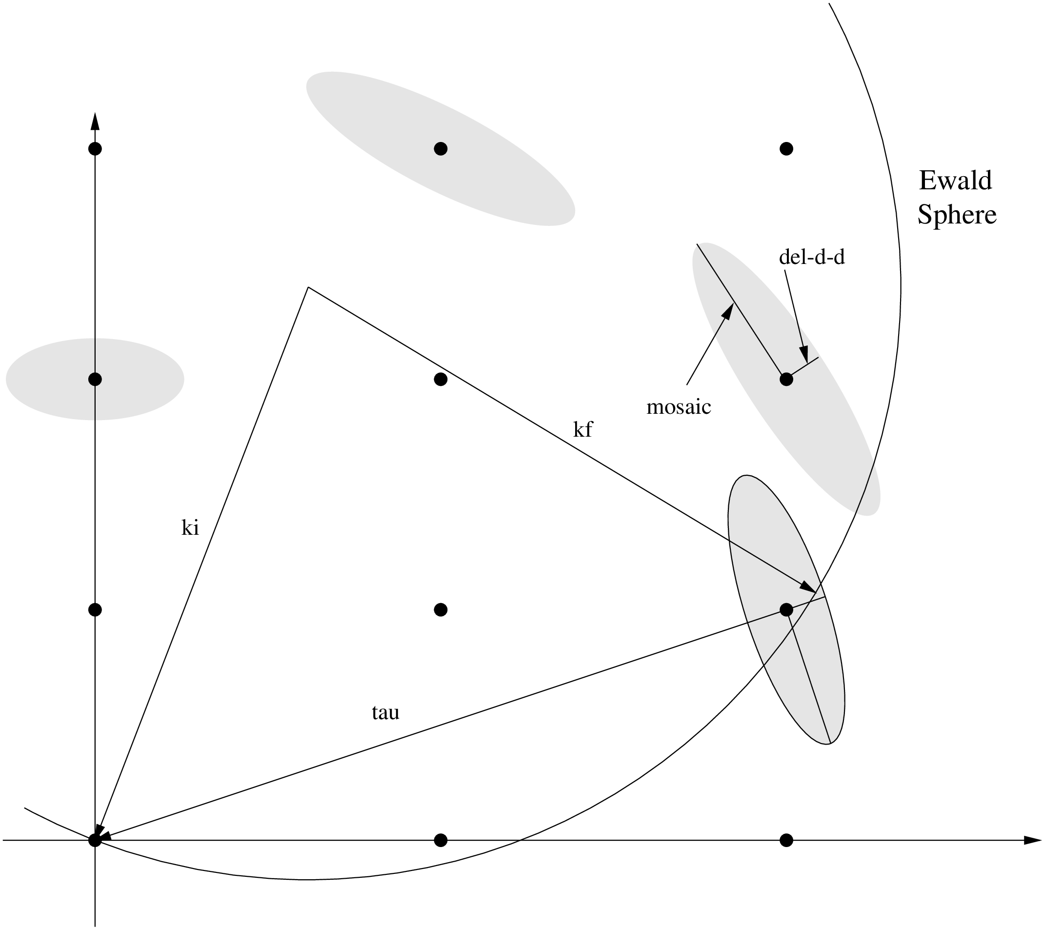
| Figure 9.4.: | Ewald sphere construction for a single neutron showing the Gaussian broadening of reciprocal lattice points in their local coordinate system. |
If the mosaic is isotropic (the same in all directions), the two Gaussian axes perpendicular to \(\boldsymbol {\tau }\) are simply arbitrary normal vectors of equal length given by the mosaic. But if the mosaic is anisotropic, the two perpendicular axes will in general be different for each scattering vector. In the absence of anything better, Single_crystal uses a model which is at least mathematically plausible and which works as expected in the two common cases: (1) isotropic mosaic, and (2) two mosaic directions (“horizontal and vertical mosaic”) perpendicular to a scattering vector.
The basis for the model is a three-dimensional Gaussian distribution in Euler angles giving the orientation probability distribution for the micro-crystals; that is, the misorientation is given by small rotations around the \(X\), \(Y\), and \(Z\) axes, with the rotation angles having (in general different) Gaussian probability distributions. For given scattering vector \(\boldsymbol {\tau }\), a rotation of the micro-crystals around an axis parallel to \(\boldsymbol {\tau }\) has no effect on the direction of the scattering vector. Suppose we form the intersection between the three-dimensional Gaussian in Euler angles and a plane through the origin perpendicular to \(\boldsymbol {\tau }\). This gives a two-dimensional Gaussian, say with axes defined by unit vectors \(\boldsymbol {g}_1\) and \(\boldsymbol {g}_2\) and mosaic widths \(\eta _1\) and \(\eta _2\).
We now let the mosaic for \(\boldsymbol {\tau }\) be defined by rotations around \(\boldsymbol {g}_1\) and \(\boldsymbol {g}_2\) with angles having Gaussian distributions of widths \(\eta _1\) and \(\eta _2\). Since \(\boldsymbol {g}_1\), \(\boldsymbol {g}_2\), and \(\boldsymbol {\tau }\) are perpendicular, a small rotation of \(\boldsymbol {\tau }\) around \(\boldsymbol {g}_1\) will change \(\boldsymbol {\tau }\) in the direction of \(\boldsymbol {g}_2\). The two axes of the Gaussian mosaic in reciprocal space that are perpendicular to \(\boldsymbol {\tau }\) will thus be given by \(\tau \eta _2\boldsymbol {g}_1\) and \(\tau \eta _1\boldsymbol {g}_2\).
We now derive a quantitative expression for the scattering cross-section of the crystal in the model. For this, we introduce a local coordinate system for each reciprocal lattice point \(\boldsymbol {\tau }\) and use \(\boldsymbol {x}\) for vectors written in local coordinates. The origin is \(\boldsymbol {\tau }\), the first axis is parallel to \(\boldsymbol {\tau }\) and the other two axes are perpendicular to \(\boldsymbol {\tau }\). In the local coordinate system, the 3-dimensional Gaussian is given by \begin {equation} \label {eq:crystal-gauss-1} G(x_1,x_2,x_3) = \frac {1}{(\sqrt {2\pi })^3}\frac {1}{\sigma _1\sigma _2\sigma _3} e^{-\frac {1}{2}(\frac {x_1^2}{\sigma _1^2} + \frac {x_2^2}{\sigma _2^2} + \frac {x_3^2}{\sigma _3^2})} \end {equation} The axes of the Gaussian are \(\sigma _1 = \tau \Delta d/d\) and \(\sigma _2 = \sigma _3 = \eta \tau \). Here we used the assumption that \(\eta \) is small, so that \(\tan \eta \approx \eta \) (with \(\eta \) given in radians). By introducing the diagonal matrix \[ D = \left ( \begin {array}[c]{ccc} \frac {1}{2}\sigma _1^2 & 0 & 0 \\ 0 & \frac {1}{2}\sigma _2^2 & 0 \\ 0 & 0 & \frac {1}{2}\sigma _3^2 \end {array}\right ) \] equation (9.16) can be written as \begin {equation} G(\boldsymbol {x}) = \frac {1}{(\sqrt {2\pi })^3}\frac {1}{\sigma _1\sigma _2\sigma _3} e^{-\boldsymbol {x}^\textrm {T} D \boldsymbol {x}} \end {equation} again with \(\boldsymbol {x}=(x_1,x_2,x_3)\) written in local coordinates.
To get an expression in the coordinates of the reciprocal lattice of the crystal, we introduce a matrix \(U\) such that if \(\boldsymbol {y} = (y_1,y_2,y_3)\) are the global coordinates of a point in the crystal reciprocal lattice, then \(U(\boldsymbol {y} + \boldsymbol {\tau })\) are the coordinates in the local coordinate system for \(\boldsymbol {\tau }\). The matrix \(U\) is given by \[ U^\textrm {T} = (\hat {u}_1, \hat {u}_2, \hat {u}_3), \] where \(\hat {u}_1\), \(\hat {u}_2\), and \(\hat {u}_3\) are the axes of the local coordinate system, written in the global coordinates of the reciprocal lattice. Thus \(\hat {u}_1 = \boldsymbol {\tau }/\tau \), and \(\hat {u}_2\) and \(\hat {u}_3\) are unit vectors perpendicular to \(\hat {u}_1\) and to each other. The matrix \(U\) is unitarian, that is \(U^{-1} = U^\textrm {T}\). The translation between global and local coordinates is \[ \boldsymbol {x} = U(\boldsymbol {y} + \boldsymbol {\tau }) \qquad \boldsymbol {y} = U^\textrm {T} \boldsymbol {x} - \boldsymbol {\tau } \]
The expression for the 3-dimensional Gaussian in global coordinates is \begin {equation} G(\boldsymbol {y}) = \frac {1}{(\sqrt {2\pi })^3}\frac {1}{\sigma _1\sigma _2\sigma _3} e^{-(U(\boldsymbol {y}+\boldsymbol {\tau }))^\textrm {T} D (U(\boldsymbol {y}+\boldsymbol {\tau }))} \end {equation} The elastic coherent cross-section is then given by \begin {equation} \label {eq:crystal-cross-section} \left (\frac {d\sigma }{d\Omega }\right )_\textrm {coh.el.} = N\frac {(2\pi )^3}{V_0}\sum _{\boldsymbol {\tau }} G(\boldsymbol {\tau } - \boldsymbol {\kappa }) |F_{\boldsymbol {\tau }}|^2 \end {equation}
9.4.2 The algorithm
The overview of the algorithm used in the Single_crystal component is as follows:
-
Check if the neutron intersects the crystal. If not, no action is taken.
-
Search through a list of reciprocal lattice points of interest, selecting those that are close enough to the Ewald sphere to have a non-vanishing scattering probability. From these, compute the total coherent cross-section \(\sigma _\textrm {coh}\) (see below), the absorption cross-section \(\sigma _\textrm {abs} = \sigma _\textrm { 2200} \frac {\textrm {2200~m/s}}{v}\), and the total cross-section \(\sigma _\textrm {tot} = \sigma _\textrm {coh}+\sigma _\textrm {inc}+\sigma _\textrm {abs}\).
-
The transmission probability is \(\exp (- \frac {\sigma _\textrm {tot}}{V_0}\ell )\) where \(\ell \) is the length of the flight path through the crystal. A Monte Carlo choice is performed to determine whether the neutron is transmitted. Optionally, the user may set a fixed Monte Carlo probability for the first scattering event, for example to boost the statistics for a weak reflection.
-
For non-transmission, the position at which the neutron will interact is selected from an exponential distribution. A Monte Carlo choice is made of whether to scatter coherently or incoherently. Absorption is treated by weight adjustment (see below).
-
For incoherent scattering, the outgoing wave vector \(\boldsymbol {k}_\textrm {f}\) is selected with a random direction.
-
For coherent scattering, a reciprocal lattice vector is selected by a Monte Carlo choice, and \(\boldsymbol {k}_\textrm {f}\) is found (see below).
-
Adjust the neutron weight as dictated by the Monte Carlo choices made.
-
Repeat from (2) until the neutron is transmitted (to simulate multiple scattering).
For point 2, the distance dist between a reciprocal lattice point and the Ewald sphere is considered small enough to allow scattering if it is less than five times the maximum axis of the Gaussian, \(\textit {dist} \leq 5\max (\sigma _1,\sigma _2,\sigma _3)\).
9.4.3 Choosing the outgoing wave vector
The final wave vector \(\boldsymbol {k}_\textrm {f}\) must lie on the intersection between the Ewald sphere and the Gaussian ellipsoid. Since \(\eta \) and \(\Delta d/d\) are assumed small, the intersection can be approximated with a plane tangential to the sphere, see figure 9.5. The tangential point is taken to lie on the line between the center of the Ewald sphere \(-\boldsymbol {k}_\textrm {i}\) and the reciprocal lattice point \(\boldsymbol {\tau }\). Since the radius of the Ewald sphere is \(k_\textrm { i}\), this point is \[ \boldsymbol {o}=(k_\textrm {i}/\rho - 1)\boldsymbol {\rho } - \boldsymbol {\tau } \] where \(\boldsymbol {\rho } = \boldsymbol {k}_\textrm {i} - \boldsymbol {\tau }\).
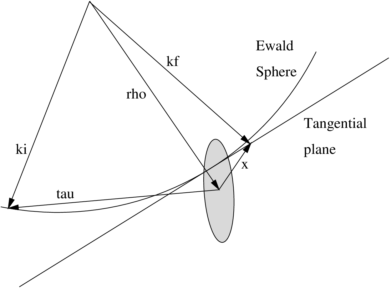
The equation for the plane is \begin {equation} \label {eq:crystal-tangent-plane} \boldsymbol {P}(\boldsymbol {t}) = \boldsymbol {o} + B \boldsymbol {t}, \qquad \boldsymbol {t} \in \mathbb {R}^2 \end {equation} Here \(B = (\boldsymbol {b}_1, \boldsymbol {b}_2)\) is a \(3\times 2\) matrix with the two generators for the plane \(\boldsymbol {b}_1\) and \(\boldsymbol {b}_2\). These are (arbitrary) unit vectors in the plane, being perpendicular to each other and to the plane normal \(\boldsymbol {n} = \boldsymbol {\rho }/\rho \).
Each \(\boldsymbol {t}\) defines a potential final wave vector \(\boldsymbol {k}_\textrm {f}(\boldsymbol {t}) = \boldsymbol {k}_\textrm {i} + \boldsymbol {P}(\boldsymbol {t})\). The value of the 3-dimensional Gaussian for this \(\boldsymbol {k}_\textrm {f}\) is \begin {equation} \label {eq:crystal-gauss-t-1} G(\boldsymbol {x}(\boldsymbol {t})) = \frac {1}{(\sqrt {2\pi })^3}\frac {1}{\sigma _1\sigma _2\sigma _3} e^{-\boldsymbol {x}(\boldsymbol {t})^\textrm {T} D \boldsymbol {x}(\boldsymbol {t})} \end {equation} where \(\boldsymbol {x}(\boldsymbol {t}) = \boldsymbol {\tau } - (\boldsymbol {k}_\textrm {i} - \boldsymbol {k}_\textrm {f}(\boldsymbol {t}))\) is given in local coordinates for \(\boldsymbol {\tau }\). It can be shown that equation (9.21) can be re-written as \begin {equation} \label {eq:crystal-gauss-2} G(\boldsymbol {x}(\boldsymbol {t})) = \frac {1}{(\sqrt {2\pi })^3}\frac {1}{\sigma _1\sigma _2\sigma _3} e^{-\alpha } e^{-(\boldsymbol {t}-\boldsymbol {t}_0)^\textrm {T} M (\boldsymbol {t}-\boldsymbol {t}_0)} \end {equation} where \(M = B^\textrm {T} D B\) is a \(2 \times 2\) symmetric and positive definite matrix, \(\boldsymbol {t}_0 = -M^{-1}B^\textrm {T} D \boldsymbol {o}\) is a 2-vector, and \(\alpha = -\boldsymbol {t}_0^\textrm {T} M \boldsymbol {t}_0 + \boldsymbol {o}^\textrm {T} D \boldsymbol {o}\) is a real number. Note that this is a two-dimensional Gaussian (not necessarily normalized) in \(\boldsymbol {t}\) with center \(\boldsymbol {t}_0\) and axis defined by \(M\).
To choose \(\boldsymbol {k}_\textrm {f}\) we sample \(\boldsymbol {t}\) from the 2-dimensional Gaussian distribution (9.22). To do this, we first construct the Cholesky decomposition of the matrix \((\frac {1}{2}M^{-1})\). This gives a \(2\times 2\) matrix \(L\) such that \(L L^\textrm {T} = \frac {1}{2}M^{-1}\) and is possible since \(M\) is symmetric and positive definite. It is given by \[ L = \left ( \begin {array}[c]{cc} \sqrt {\nu _{11}} & 0 \\ \frac {\nu _{12}}{\sqrt {\nu _{11}}} & \sqrt {\nu _{22} - \frac {\nu _{12}^2}{\nu _{11}}} \end {array}\right ) \qquad \hbox {where } \frac {1}{2}M^{-1} = \left ( \begin {array}[c]{cc} \nu _{11} & \nu _{12} \\ \nu _{12} & \nu _{22} \end {array}\right ) \] Now let \(\boldsymbol {g} = (g_1, g_2)\) be two random numbers drawn form a Gaussian distribution with mean 0 and standard deviation 1, and let \(\boldsymbol {t} = L\boldsymbol {g} + \boldsymbol {t}_0\). The probability of a particular \(\boldsymbol {t}\) is then
where we used that \(\boldsymbol {g}=L^{-1}(\boldsymbol {t}-\boldsymbol {t}_0)\) so that \(d\boldsymbol {g} = \frac {1}{\det L}d\boldsymbol {t}\). This is just the normalized form of (9.22). Finally we set \(\boldsymbol {k}'_\textrm {f} = \boldsymbol {k}_\textrm {i} + \boldsymbol {P}(\boldsymbol {t})\) and \(\boldsymbol {k}_\textrm {f} = (k_\textrm {i}/k'_f)\boldsymbol {k}'_\textrm {f}\) to normalize the length of \(\boldsymbol {k}_\textrm {f}\) to correct for the (small) error introduced by approximating the Ewald sphere with a plane.
9.4.4 Computing the total coherent cross-section
To determine the total coherent scattering cross-section, the differential cross-section must be integrated over the Ewald sphere: \[ \sigma _\textrm {coh} = \int _\textrm {Ewald} \left (\frac {d\sigma }{d\Omega }\right )_\textrm {coh.el.} d\Omega \] For small mosaic we may approximate the sphere with the tangential plane, and we thus get from (9.19) and (9.22):
As before, we let \(\boldsymbol {g} = L^{-1}(\boldsymbol {t} - \boldsymbol {t}_0)\) so that \(d\boldsymbol {t} = \det (L) d\boldsymbol {g}\).
Neutron weight factor adjustment
We now calculate the correct neutron weight adjustment for the Monte Carlo choices made. In three cases is a Monte Carlo choice made with a probability different from the probability of the corresponding physical event: When deciding whether to transmit the neutron or not, when simulating absorption, and when selecting the reciprocal lattice vector \(\boldsymbol {\tau }\) to scatter from.
If the user has choosen a fixed transmission probability \(f(\textrm { transmit}) = p_\textrm {transmit}\), the neutron weight must be adjusted by \[ \pi (\textrm {transmit}) = \frac {P(\textrm {transmit})}{f(\textrm {transmit})} \] where \(P(\textrm {transmit}) = \exp (-\frac {\sigma _\textrm {tot}}{V_0}\ell )\) is the physical transmission probability. Likewise, for non-transmission the adjustment is \[ \pi (\textrm {no~transmission}) = \frac {1-P(\textrm {transmit})}{1-f(\textrm {transmit})}. \]
Absorption is never explicitly simulated, so the Monte Carlo probability of coherent or incoherent scattering is \(f(\textrm {coh})+f(\textrm {inc}) = 1\). The physical probability of coherent or incoherent scattering is \[ P(\textrm {coh})+P(\textrm {inc}) = \frac {\sigma _\textrm {coh} + \sigma _\textrm { inc}}{\sigma _\textrm {tot}}, \] so again a weight adjustment \(\pi (\textrm {coh}|\textrm {inc}) = \Pi (\textrm { coh}|\textrm {inc})/f(\textrm {coh}|\textrm {inc})\) is needed.
When choosing the reciprocal lattice vector \(\boldsymbol {\tau }\) to scatter from, the relative probability for \(\boldsymbol {\tau }\) is \(r_{\boldsymbol {\tau }} = \sigma _{\textrm { coh},\boldsymbol {\tau }}/|F_{\boldsymbol {\tau }}|^2\). This is done to get better statistics for weak reflections. The Monte Carlo probability for the reciprocal lattice vector \(\boldsymbol {\tau }\) is thus \[ f(\boldsymbol {\tau }) = \frac {r_{\boldsymbol {\tau }}}{\sum _{\boldsymbol {\tau }} r_{\boldsymbol {\tau }}} \] whereas the physical probability is \(P(\boldsymbol {\tau }) = \sigma _{\textrm { coh},\boldsymbol {\tau }}/\sigma _\textrm {coh}\). A weight adjustment is thus needed of \[ \pi (\boldsymbol {\tau }) = \frac {P(\boldsymbol {\tau })}{f(\boldsymbol {\tau })} = \frac {\sigma _{\textrm {coh},\boldsymbol {\tau }} \sum _{\boldsymbol {\tau }} r_{\boldsymbol {\tau }}} {\sigma _\textrm {coh} \; r_{\boldsymbol {\tau }}}.\]
In most cases, however, only one reflection is possible, whence \(\pi =1\).
9.4.5 Implementation details
The equations describing Single_crystal are quite complex, and consequently the code is fairly sizeable. Most of it is just the expansion of the vector and matrix equations in individual coordinates, and should thus be straightforward to follow.
The implementation pre-computes a lot of the necessary values in the INITIALIZE section. It is thus actually very efficient despite the complexity. If the list of reciprocal lattice points is big, however, the search through the list will be slow. The precomputed data is stored in the structures hkl_info and in an array of hkl_data structures (one for each reciprocal lattice point in the list). In addition, for every neutron event an array of tau_data is computed with one element for each reciprocal lattice point close to the Ewald sphere. Except for the search for possible \(\boldsymbol {\tau }\) vectors, all computations are done in local coordinates using the matrix \(U\) to do the necessary transformations.
The list of reciprocal lattice points is specified in an ASCII data file. Each line contains seven numbers, separated by white space. The first three numbers are the \((h,k,l)\) indices of the reciprocal lattice point, and the last number is the value of the structure factor \(|F_{\boldsymbol {\tau }}|^2\), in barns. The middle three numbers are not used and may be omitted; they are nevertheless recommended since this makes the file format compatible with the output from the Crystallographica program [Cry]. Any line beginning with any character of #;/% is considered to be a comment, and lines which can not be read as vectors/matrices are ignored.
The column signification may also explicitely be set in the data file header using any of the lines:
1  #column_h <index of the Bragg Qh column>
2  #column_k <index of the Bragg Qk column>
3  #column_l <index of the Bragg Ql column>
4  #column_F2 <index of the squared str. factor ’|F|^2’ column [b]>
5  #column_F  <index of the structure factor norm ’|F|’ column>
Other component parameters may as well be specified in the data file header with lines e.g.:
1  #sigma_abs <value of Absorption cross section [barns]>
2  #sigma_inc <value of Incoherent cross section [barns]>
3  #Delta_d/d <value of Delta_d/d width for all lines>
4  #lattice_a <value of the a lattice parameter [Angs]>
5  #lattice_a <value of the b lattice parameter [Angs]>
6  #lattice_a <value of the c lattice parameter [Angs]>
7  #lattice_aa <value of the alpha lattice angle [deg]>
8  #lattice_bb <value of the beta  lattice angle [deg]>
9  #lattice_cc <value of the gamma lattice angle [deg]>
Example data *.lau files are given in directory MCSTAS/data.
These files contain an extensive self-documented header defining most the sample parameters, so that only the file name and mosaicity should be given to the component:
1  Single_crystal(xwidth=0.01, yheight=0.01, zdepth=0.01,
2    mosaic = 5, reflections="YBaCuO.lau")
Powder files from ICSD/LAZY [Ics] and Fullprof [Ful] may also be used (see Table 1.2, page 50). We do not recommend to use these as the equivalent \(\vec q\) vectors are superposed, not all Bragg spots will be simulated, and the intensity will not be scaled by the multiplicity for each spot.