8.1  The Monochromator_flat McStas Component

Flat Monochromator crystal with anisotropic mosaic.

Identification

• Author: Kristian Nielsen

• Origin: Risoe

• Date: 1999

Description

Flat, infinitely thin mosaic crystal, useful as a monochromator or analyzer. For an unrotated monochromator component, the crystal surface lies in the Y-Z plane (ie. parallel to the beam). The mosaic is anisotropic gaussian, with different FWHMs in the Y and Z directions. The scattering vector is perpendicular to the surface.

Example: Monochromator_flat(zmin=-0.1, zmax=0.1, ymin=-0.1, ymax=0.1, mosaich=30.0, mosaicv=30.0, r0=0.7, Q=1.8734)

Monochromator lattice parameter

PG       002 DM=3.355 AA (Highly Oriented Pyrolythic Graphite)
PG       004 DM=1.677 AA

Heusler 111 DM=3.362 Å (Cu2MnAl)

CoFe         DM=1.771 AA (Co0.92Fe0.08)
Ge       111 DM=3.266 AA
Ge       311 DM=1.714 AA
Ge       511 DM=1.089 AA
Ge       533 DM=0.863 AA
Si       111 DM=3.135 AA
Cu       111 DM=2.087 AA
Cu       002 DM=1.807 AA
Cu       220 DM=1.278 AA
Cu       111 DM=2.095 AA

Input parameters

Parameters in boldface are required; the others are optional.

Links

• Component source code found in file Monochromator_flat.comp.

An infinitely thin, flat mosaic crystal with a single scattering vector

This component simulates an infinitely thin single crystal with a single scattering vector, \(Q_0=2\pi / d_m\), perpendicular to the surface. A typical use for this component is to simulate a simple monochromator or analyzer.

The monochromator dimensions are given by the length, \(z_\textrm {w}\), and the height, \(y_\textrm {h}\). As the parameter names indicate, the monochromator is placed in the \(z-y\) plane of the local coordinate system. This definition is made to ensure that the physical monochromator angle (often denoted A1) will equal the McStas rotation angle of the Monochromator component around the \(y\)-axis. \(R_0\) is the maximal reflectivity and \(\eta _\textrm {h}\) and \(\eta _\textrm {v}\) are the horizontal and vertical mosaicities, respectively, see explanation below.

Monochromator physics and algorithm

The physical model used in Monochromator_flat is a rectangular piece of material composed of a large number of small micro-crystals. The orientation of the micro-crystals deviates from the nominal crystal orientation so that the probability of a given micro-crystal orientation is proportional to a Gaussian in the angle between the given and the nominal orientation. The width of the Gaussian is given by the mosaic spread, \(\eta \), of the crystal (given in units of arc minutes). \(\eta \) is assumed to be large compared to the inherent Bragg width of the scattering vector (often a few arc seconds). (The mosaicity gives rise to a Gaussian reflectivity profile of width similar to - but not equal - the intrinsic mosaicity. In this component, and in real life, the mosaicity given is that of the reflectivity signal.)

As a further simplification, the crystal is assumed to be infinitely thin. This means that multiple scattering effects are not simulated. It also means that the total reflectivity, \(r_0\) is used as a parameter for the model rather than the atomic scattering cross section, implying that the scattering efficiency does not vary with neutron wavelength. The variance of the lattice spacing (\(\Delta d/d\)) is assumed to be zero, so this component is not suitable for simulating backscattering instruments (use the component Single_crystal in section 9.4 for that).

When a neutron trajectory intersects the crystal, the first step in the computation is to determine the probability of scattering. This probability is then used in a Monte Carlo choice deciding whether to scatter or transmit the neutron. The physical scattering probability is the sum of the probabilities of first- second-, and higher-order scattering - up to the highest order possible for the given neutron wavelength. However, in most cases at most one order will have a significant scattering probability, and the computation thus considers only the order that best matches the neutron wavelength.

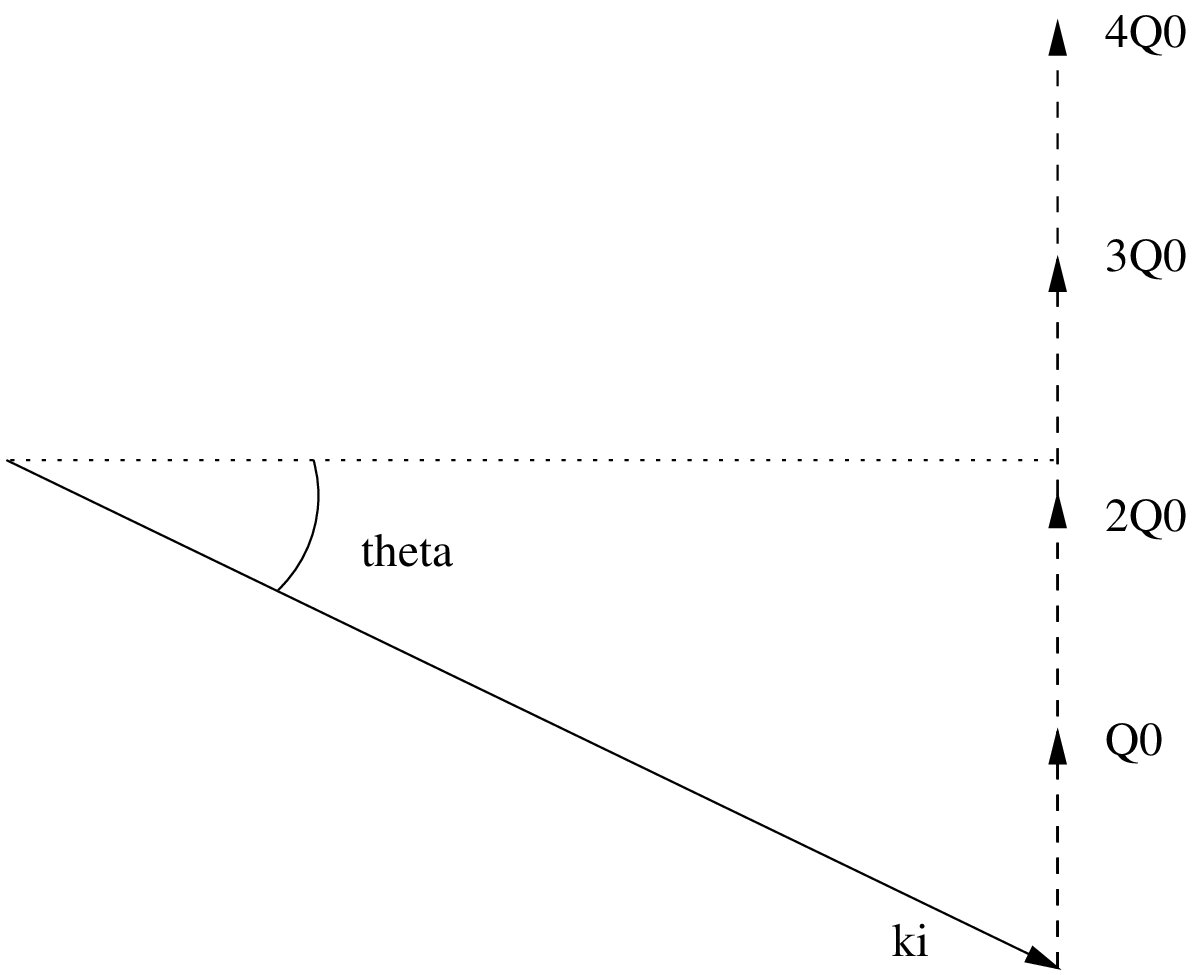
The scattering of neutrons from a crystal is governed by Bragg’s law: \begin {equation} n\textbf {Q}_0 = 2\textbf {k}_i\sin \theta \end {equation} The scattering order is specified by the integer \(n\). We seek only one value of \(n\), namely the one which makes \(n \textbf {Q}_0\) closest to the projection of \(2\textbf {k}_i\) onto \(\textbf {Q}_0\) (see figure 8.1).

Once \(n\) has been determined, the Bragg angle \(\theta \) can be computed. The angle \(\alpha \) is the amount one would need to turn the nominal scattering vector \(\textbf {Q}_0\) for the monochromator to be in Bragg scattering condition. We now use \(\alpha \) to compute the probability of reflection from the mosaic crystal \begin {equation} p_\textrm {reflect} = R_0 e^{-\alpha ^2/2\eta ^2}, \end {equation} The probability \(p_\textrm {reflect}\) is used in a Monte Carlo choice to decide whether the neutron is transmitted or reflected.

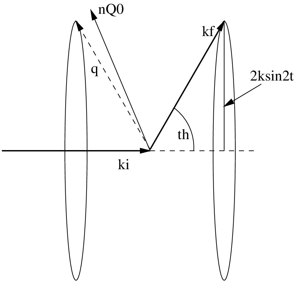
In the case of reflection, the neutron will be scattered into the Debye-Scherrer cone, with the probability of each point on the cone being determined by the mosaic. The Debye-Scherrer cone can be described by the equation \begin {equation} \label {eq:mosaic_cone} \textbf {k}_\textrm {f} = \textbf {k}_\textrm {i}\cos 2\theta + \sin 2\theta (\textbf {c}\cos \varphi + \textbf {b}\sin \varphi ), \qquad \varphi \in [-\pi ;\pi ], \end {equation} where \(\textbf {b}\) is a vector perpendicular to \(\textbf {k}_\textrm {i}\) and \(\textbf { Q}_0\), \(\textbf {c}\) is perpendicular to \(\textbf {k}_\textrm {i}\) and \(\textbf {b}\), and both \(\textbf {b}\) and \(\textbf {c}\) have the same length as \(\textbf {k}_\textrm {i}\) (see figure 8.2). When choosing \(\varphi \) (and thereby \(\textbf {k}_\textrm {f}\)), only a small part of the full \([-\pi ; \pi ]\) range will have appreciable scattering probability in non-backscattering configurations. The best statistics is thus obtained by sampling \(\varphi \) only from a suitably narrow range.

The (small) deviation angle \(\alpha \) of the nominal scattering vector \(n\textbf {Q}_0\) corresponds to a \(\Delta q\) of \begin {equation} \Delta q \approx \alpha 2k\sin \theta . \end {equation} The angle \(\varphi \) corresponds to a \(\Delta k_\textrm {f}\) (and hence \(\Delta q\)) of \begin {equation} \Delta q \approx \varphi k \sin (2\theta ) \end {equation} (see figure 8.2). Hence we may sample \(\varphi \) from a Gaussian with standard deviation \begin {equation} \alpha \frac {2k\sin \theta }{k\sin (2\theta )} = \alpha \frac {2k\sin \theta }{2k\sin \theta \cos \theta } = \frac {\alpha }{\cos \theta } \end {equation} to get good statistics.

What remains is to determine the neutron weight. The distribution from which the scattering event is sampled is a Gaussian in \(\varphi \) of width \(\frac {\alpha }{\cos \theta }\), \begin {equation} f_\textrm {MC}(\varphi ) = \frac {1}{\sqrt {2\pi }(\sigma /\cos \theta )} e^{-\varphi ^2/2(\sigma /\cos \theta )^2} \end {equation} In the physical model, the probability of the scattering event is proportional to a Gaussian in the angle between the nominal scattering vector \(\textbf {Q}_0\) and the actual scattering vector \(\textbf {q}\). The normalization condition is that the integral over all \(\varphi \) should be 1. Thus the probability of the scattering event in the physical model is \begin {equation} \label {eq:mosaic_integral} \Pi (\varphi ) = e^{\frac {-d(\varphi )^2}{2\sigma ^2}} / \int _{-\pi }^{\pi } e^{\frac {-d(\varphi )^2}{2\sigma ^2}} d\varphi \end {equation} where \(d(\varphi )\) denotes the angle between the nominal scattering vector and the actual scattering vector corresponding to \(\varphi \). According to equation (2.9), the weight adjustment \(\pi _j\) is then given by \begin {equation} \pi _j = \Pi (\varphi ) / f_\textrm {MC}(\varphi ). \end {equation} In the implementation, the integral in (8.8) is computed using a 15-order Gaussian quadrature formula, with the integral restricted to an interval of width \(5\sigma /\cos \theta \) for the same reasons discussed above on the sampling of \(\varphi \).