9 Samples
This class of components models the sample of the experiment. This is by far the most challenging part of a neutron scattering instrument to model. However, for purpose of simulating instrument performance, details of the samples are rather unimportant, allowing for simple approximations. On the contrary, for full virtual experiments it is of importance to have realistic and detailed sample descriptions. McStas contains both simple and detailed samples.
We first consider incoherent scattering. The general-purpose Incoherent component performs incoherent scattering and absorption for an arbitrary shape; the older, simpler V_sample component that previously served this role has moved to the obsolete component category (see the Component Manual’s Obsolete chapter) and is superseded by Incoherent.
An important component class is elastic Bragg scattering from an ideal powder. The component PowderN models a powder scatterer with reflections given in an input file. To scatter on a single Bragg peak, the Powder1 component may be used. The component includes absorption, incoherent scattering, direct beam transmission and can assume concentric shape, i.e. can be used for modelling sample enviroments.
Next type is Bragg scattering from single crystals. The simplest single crystals are in fact the monochromator components like Monochromator_flat, presented in section 8.1. The monochromators are models of a thin mosaic crystal with a single scattering vector perpendicular to the surface. Much more advanced, the component Single_crystal is a general single crystal sample (with multiple scattering) that allows the input of an arbitrary unit cell and a list of structure factors, read from a LAZY / Crystallographica file. This component also allows anisotropic mosaicity and \(\Delta d/d\) lattice space variation.
Isotropic small-angle scattering is simulated in Sans_Spheres, which models scattering from a collection of hard spheres (dilute colloids).
Inelastic scattering from a dispersion is exemplified by the component Phonon_simple, which models scattering from a single acoustic phonon branch.
For a more general sample model, the Isotropic_Sqw component is able to simulate all kinds of isotropic materials: Liquids, glasses, polymers, powders, etc, with \(S(q,\omega )\) table specified by an input file. Physical processes include coherent/incoherent scattering, both elastic and inelastic, with absorption and multiple scattering. Moreover, this component may be used concentrically, to model a sample environment. Thus it may handle most samples except single crystals.
| Sample | Coherent | Incoherent | ||||
| Process | Elastic | Inelastic | Elastic | Inelastic | Absorption | Multi. Scatt. |
| Phonon_simple | X | 1 | ||||
| Isotropic_Sqw | X | X | X | X | 2 | X |
| Powder1 | 1 line | X | 1 | |||
| PowderN | N lines | X | 1 | |||
| Sans_spheres | colloid | 1 | ||||
| Single_crystal | X | X | 2 | X | ||
| V_sample | X | QE broad. | 1 | |||
| Tunneling_sample | X | X | QE broad. | 1 | ||
| Table 9.1.: | Processes implemented in sample components. Absorption: 1=single only, 2=with secondary |
9.0.2 Weight transformation in samples; focusing
9.0.3 Small-angle scattering (SANS) and other sample models
9.1 The Incoherent McStas Component
Identification
Description
Input parameters
Links
An incoherent scatterer, the V-sample
9.1.1 Physics and algorithm
9.1.2 Remark on functionality
9.2 The Tunneling_sample McStas Component
Identification
Description
Input parameters
Links
An incoherent inelastic scatterer
9.3 The PowderN McStas Component
Identification
Description
Input parameters
Links
A general powder sample
9.3.1 Files formats: powder structures
9.3.2 Geometry, physical properties, concentricity
9.3.3 Powder scattering
9.3.4 Algorithm
9.4 The Single_crystal McStas Component
Identification
Description
Input parameters
Links
The single crystal component
9.4.1 The physical model
9.4.2 The algorithm
9.4.3 Choosing the outgoing wave vector
9.4.4 Computing the total coherent cross-section
9.4.5 Implementation details
9.5 The Sans_spheres McStas Component
Identification
Description
Input parameters
Links
A sample of hard spheres for small-angle scattering
9.5.1 Small-angle scattering cross section
9.5.2 Algorithm
9.5.3 Calculating the weight factor
9.6 The Phonon_simple McStas Component
Identification
Description
Input parameters
Links
A simple phonon sample
9.6.1 The phonon cross section
9.6.2 The algorithm
9.6.3 The weight transformation
9.7 The Isotropic_Sqw McStas Component
Identification
Description
Input parameters
Links
A general \(S(q,\omega )\) coherent and incoherent scatterer
9.7.1 Neutron interaction with matter - overview
9.7.2 Theoretical side
9.7.3 Theoretical side - scattering in the sample
9.7.4 The implementation
9.7.5 Validation
9.8 Samples for resolution-function calculations
9.9 The Res_sample McStas Component
Identification
Description
Input parameters
Links
9.10 The TOFRes_sample McStas Component
Identification
Description
Input parameters
Links
9.0.1 Neutron scattering notation
In sample components, we use the notation common for neutron scattering, where the wave vector transfer is denoted the scattering vector \begin {equation} \label {eq:q-transfer} \textbf {q} \equiv \textbf {k}_\textrm {i} - \textbf {k}_\textrm {f} . \end {equation} In analygo, the energy transfer is given by \begin {equation} \label {eq:w-transfer} \hbar \omega \equiv E_\textrm {i} - E_\textrm {f} = \frac {\hbar ^2}{2 m_\textrm {n}} \left ( k_\textrm {i}^2 - k_\textrm {f}^2 \right ) . \end {equation}
9.0.2 Weight transformation in samples; focusing
Within many samples, the incident beam is attenuated by scattering and absorption, so that the illumination varies considerably throughout the sample. For single crystals, this phenomenon is known as secondary extinction [Bac75], but the effect is important for all samples. In analytical treatments, attenuation is difficult to deal with, and is thus often ignored, making a thin sample approximation. In Monte Carlo simulations, the beam attenuation is easily taken care of, as will be shown below. In the description, we ignore multiple scattering, which is however implemented in some sample components.
The sample has an absorption cross section per unit cell of \(\sigma _c^a\) and a scattering cross section per unit cell of \(\sigma _c^s\). The neutron path length in the sample before the scattering event is denoted by \(l_1\), and the path length within the sample after the scattering is denoted by \(l_2\), see figure 9.1. We then define the inverse penetration lengths as \(\mu ^s = \sigma _c^s / V_c\) and \(\mu ^a = \sigma _c^a / V_c\), where \(V_c\) is the volume of a unit cell. Physically, the attenuation along this path follows \begin {equation} f_\textrm {att}(l) = \exp (- l (\mu ^s + \mu ^a)) , \end {equation} where the normalization \(f_\textrm {att}(0)=1\).
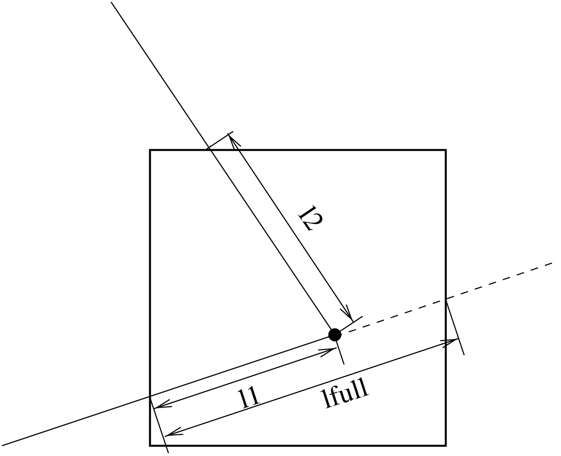
The probability for a given neutron ray to be scattered from within the interval \([ l_1 ; l_1+dl ]\) will be \begin {equation} P(l_1) dl = \mu ^s f_\textrm {att}(l_1) dl , \end {equation} while the probability for a neutron to be scattered from within this interval into the solid angle \(\Omega \) and not being scattered further or absorbed on the way out of the sample is \begin {equation} P(l_1,\Omega ) dl d\Omega = \mu ^s f_\textrm {att}(l_1) f_\textrm {att}(l_2) \gamma (\Omega ) d\Omega dl , \end {equation} where \(\gamma (\Omega )\) is the directional distribution of the scattered neutrons, and \(l_2\) is determined by Monte Carlo chocies of \(l_1\), \(\Omega \), and from the sample geometry, see e.g. figure 9.1.
In our Monte-Carlo simulations, we may choose the scattering parameters by making a Monte-Carlo choice of \(l_1\) and \(\Omega \) from a distribution different from \(P(l_1,\Omega )\). By doing this, we must adjust \(\pi _i\) according to the probability transformation rule (2.9). If we e.g. choose the scattering depth, \(l_1\), from a flat distribution in \([ 0 ; l_\textrm {full} ]\), and choose the directional dependence from \(g(\Omega )\), we have a Monte Carlo probability \begin {equation} f(l_1,\Omega ) = g(\Omega ) / l_\textrm {full} , \end {equation} \(l_\textrm {full}\) is here the path length through the sample as taken by a non-scattered neutron (although we here assume that all simulated neutrons are being scattered). According to (2.9), the neutron weight factor is now adjusted by the amount \begin {equation} \label {sampleprob} \pi _i(l_1,\Omega ) = \mu ^s l_\textrm {full} \exp \left [ - (l_1+l_2) (\mu ^a + \mu ^s) \right ] \frac {\gamma (\Omega )}{g(\Omega )} . \end {equation}
In analogy with the source components, it is possible to define "interesting" directions for the scattering. One will then try to focus the scattered neutrons, choosing a \(g(\Omega )\), which peaks around these directions. To do this, one uses (9.7), where the fraction \(\gamma (\Omega )/g(\Omega )\) corrects for the focusing. One must choose a proper distribution so that \(g(\Omega ) > 0\) in every interesting direction. If this is not the case, the Monte Carlo simulation gives incorrect results. All samples have been constructed with a focusing and a non-focusing option.
9.0.3 Small-angle scattering (SANS) and other sample models
Beyond the simple isotropic small-angle model Sans_spheres (scattering from a dilute collection of hard spheres), McStas provides two further, much richer routes to SANS sample modelling:
-
native McStas SANS models contributed in the contrib category (SANSSpheres, SANSCylinders, SANSNanodiscs, SANSPDB, and many others – see the Component Manual’s Contributed Components chapter), several with polydisperse and multiple-scattering variants;
-
the sasmodels category (see the Component Manual’s dedicated chapter), exposing the same, actively maintained SANS/USANS form-factor library used for data fitting in SasView, via the generic SasView_model interface.
In general, all samples are assumed to be homogeneous. There is potential in developing inhomogeneous samples, e.g. with a spatially varying lattice constant (relevant for stress/strain scanners) or inhomogeneous absorption (relevant for tomography), and reflectometry sample models beyond Multilayer_Sample (contrib). Polarization effects are handled by a dedicated set of polarisation-aware optics and field components rather than the samples described in this chapter – see the Polarisation chapter, 15.14.